Load packages and data
This vignette shows different ways on how to plot WATLAS data. Each chunk of code only requires this chunk with loading the data to be run before and is otherwise independent.
# Packages
library(tools4watlas)
library(data.table)
library(ggplot2)
library(viridis)
library(RColorBrewer)
Using ggplot2 and a basemap layer
We can create simple base maps of the study area by using the
function atl_create_bm(). This function uses a data.table
with x- and y-coordinates to check the required bounding box (which can
be extended with a buffer in meters) and spatial features (polygons) of
land, lakes, mudflats and rivers. Without adding costmized data, it will
default to the data provided in the package. By changing
asp the desired aspect ratio can be chosen (default is
“16:9”). If no data are provided the function creates a map around
Griend with a specified buffer.
Map with points and tracks of one individual
# Load example data
data <- data_example

# Subset bar-tailed godwit
data_subset <- data[species == "bar-tailed godwit"]

# Create base map
bm <- atl_create_bm(data_subset, buffer = 800)

# Plot points and tracks
bm +
  geom_path(
    data = data_subset, aes(x, y, colour = tag),
    alpha = 0.1, show.legend = FALSE
  ) +
  geom_point(
    data = data_subset, aes(x, y, colour = tag),
    size = 0.5, show.legend = FALSE
  ) +
  scale_color_brewer(palette = "Dark2") # for up to 8 categories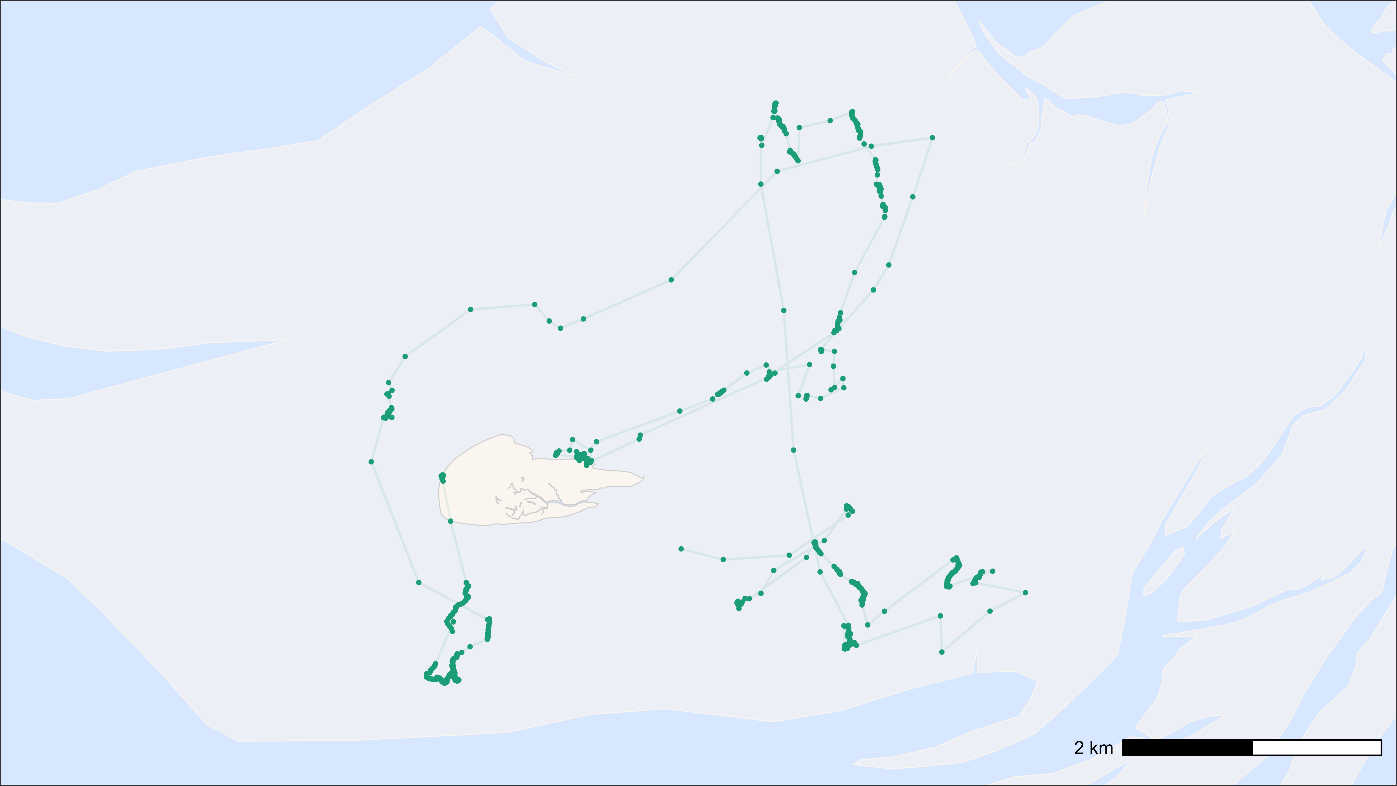
Points and tracks on basemap
Map with points and tracks of multiple species
# Create base map
bm <- atl_create_bm(data, buffer = 800)

# Plot points and tracks
bm +
  geom_path(
    data = data, aes(x, y, colour = species),
    alpha = 0.5, show.legend = FALSE
  ) +
  geom_point(
    data = data, aes(x, y, color = species),
    size = 1, show.legend = TRUE
  ) +
  scale_color_manual(
    values = atl_spec_cols(),
    labels = atl_spec_labs("multiline"),
    name = ""
  ) +
  guides(colour = guide_legend(
    nrow = 1, override.aes = list(size = 7, pch = 16, alpha = 1)
  )) +
  theme(
    legend.position = "top",
    legend.justification = "center",
    legend.key = element_blank(),
    legend.background = element_rect(fill = "transparent")
  )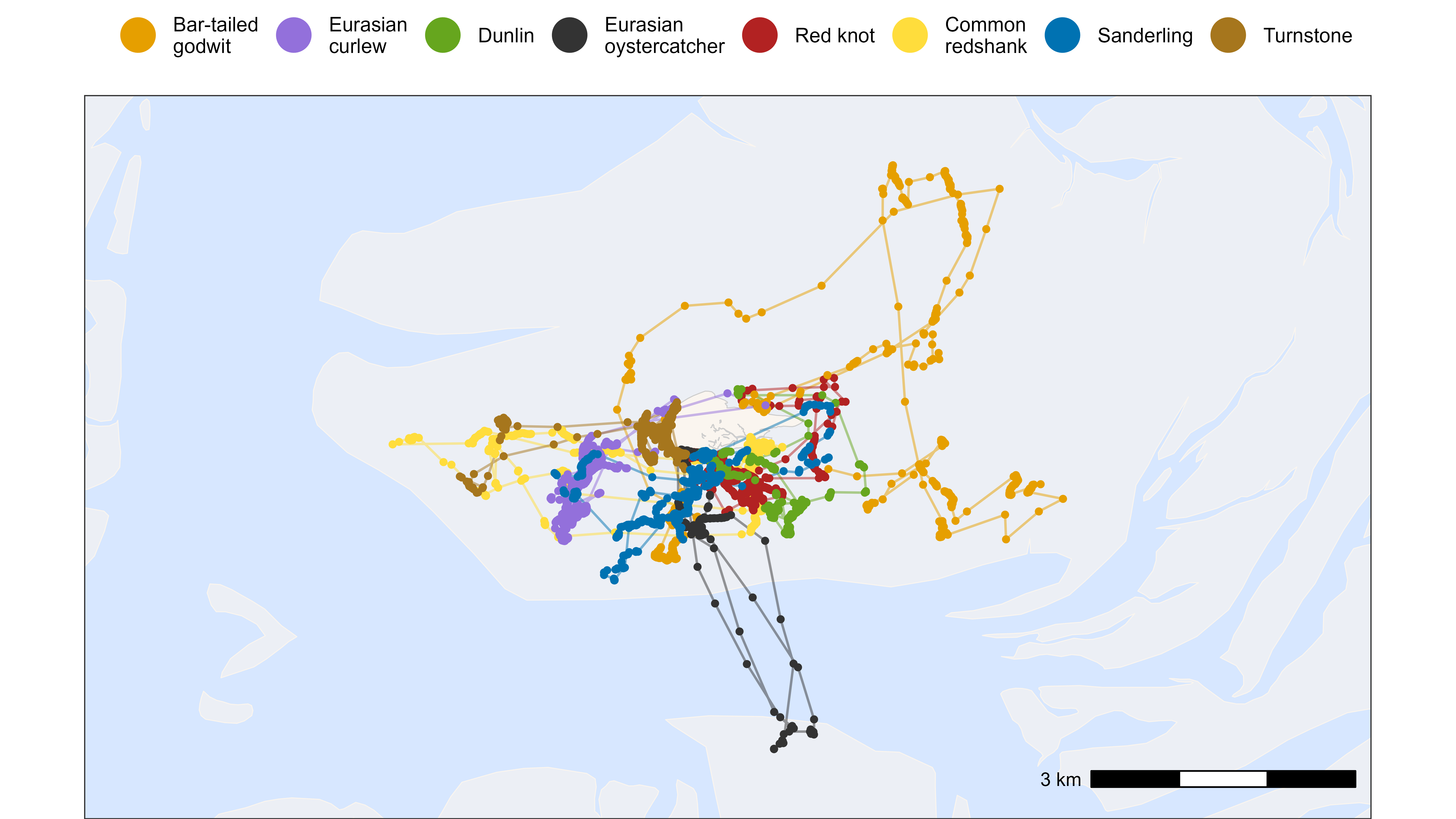
Points and tracks of multiple species on basemap
Heatmap of all positions
library(scales)

# Round data to 200 m grid cells
data_heatmap <- copy(data)
data_heatmap[, c("x_round", "y_round") := list(
  plyr::round_any(x, 200),
  plyr::round_any(y, 200)
)]
data_heatmap <- data_heatmap[, .N, by = c("x_round", "y_round")]

# Plot heatmap
bm +
  geom_tile(
    data = data_heatmap, aes(x_round, y_round, fill = N),
    linewidth = 0.1, show.legend = TRUE
  ) +
  scale_fill_viridis(
    option = "A", discrete = FALSE, trans = "log10", name = "N positions",
    breaks = trans_breaks("log10", function(x) 10^x),
    labels = trans_format("log10", math_format(10^.x)),
    direction = -1
  )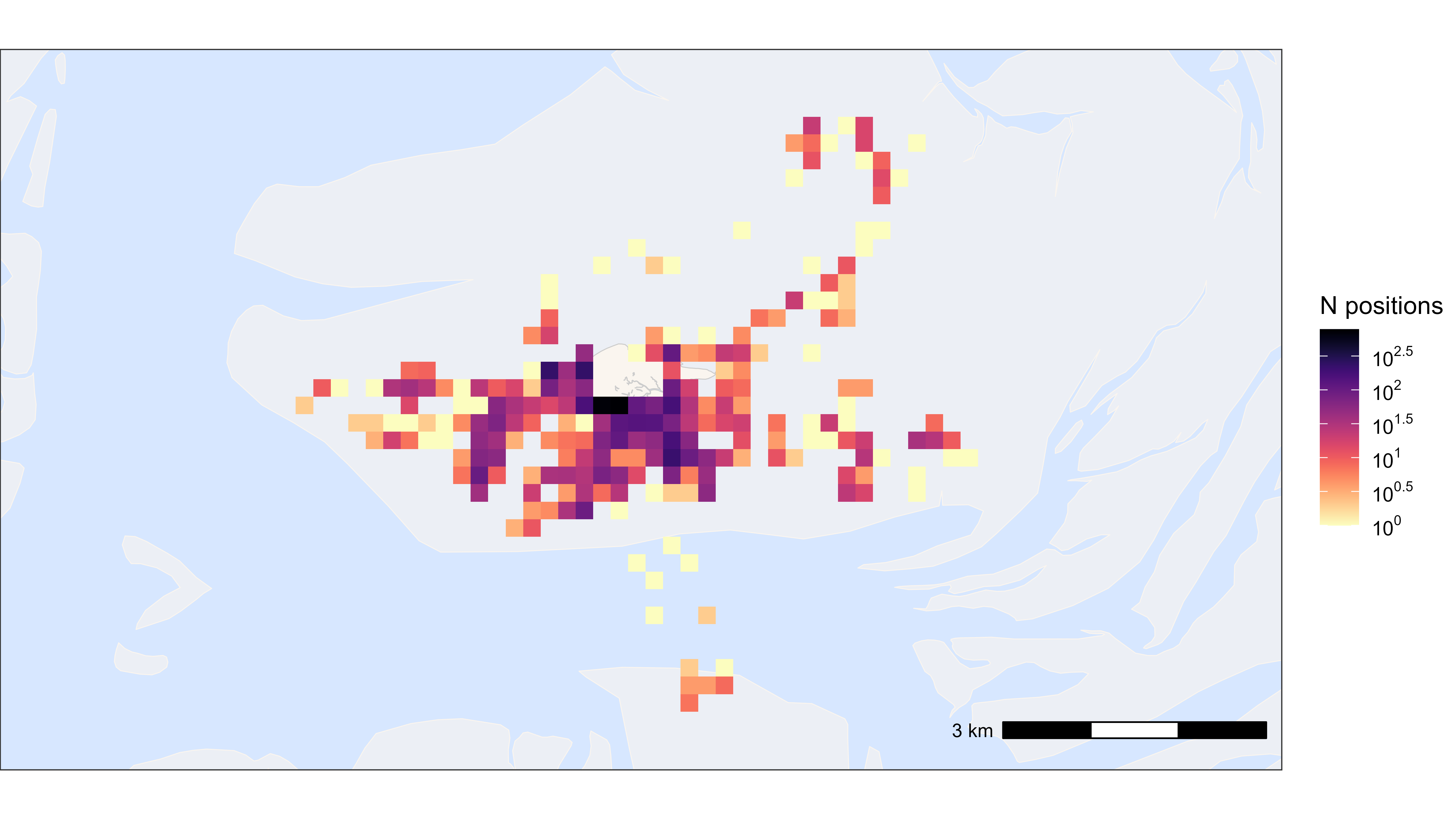
Heatmap of all positions
Interactive leaflet map with mapview
This is useful when manually checking specific data. Check for more details the mapview website. Nopte that one can change the base map by clicking in the layer symbol, to for example a satellite image.
library(mapview)
library(sf)

# make data spatial
d_sf <- atl_as_sf(data, additional_cols = c("datetime", "species"))

# add track
d_sf_lines <- atl_as_sf(data,
  additional_cols = c("species"),
  option = "lines"
)

# Plot interactive map
mapview(d_sf_lines, zcol = "species", legend = FALSE) +
  mapview(d_sf, zcol = "species")
Static map with OpenStreetMap
library(OpenStreetMap)
library(sf)

# make data spatial and transform projection to WGS 84 (used in osm)
d_sf <- atl_as_sf(data, additional_cols = c("tag", "datetime"))
d_sf <- st_transform(d_sf, crs = st_crs(4326))

# get bounding box
bbox <- atl_bbox(d_sf, asp = "16:9", buffer = 500)

# extract openstreetmap
# other 'type' options are "osm", "maptoolkit-topo", "bing", "stamen-toner",
# "stamen-watercolor", "esri", "esri-topo", "nps", "apple-iphoto", "skobbler";
map <- openmap(
  c(bbox["ymax"], bbox["xmin"]),
  c(bbox["ymin"], bbox["xmax"]),
  type = "bing", mergeTiles = TRUE
)

bm <- autoplot.OpenStreetMap(map)

# transform points to Mercator and add transformed coordinates to data
d_sf <- st_transform(d_sf, crs = sf::st_crs(3857))
osm_coords <- st_coordinates(d_sf)
data[, `:=`(x_osm = osm_coords[, 1], y_osm = osm_coords[, 2])]

# plot
bm +
  geom_path(
    data = data, aes(x_osm, y_osm, colour = species), alpha = 0.1,
    show.legend = FALSE
  ) +
  geom_point(
    data = data, aes(x_osm, y_osm, colour = species), size = 0.5,
    show.legend = TRUE
  ) +
  scale_color_manual(
    values = atl_spec_cols(),
    labels = atl_spec_labs("multiline"),
    name = ""
  ) +
  guides(colour = guide_legend(
    nrow = 1, override.aes = list(size = 7, pch = 16, alpha = 1)
  )) +
  theme(
    legend.position = "top",
    legend.justification = "center",
    legend.key = element_blank(),
    legend.background = element_rect(fill = "transparent")
  ) +
  labs(x = "Longitude", y = "Latitude") +
  coord_sf(crs = 3857)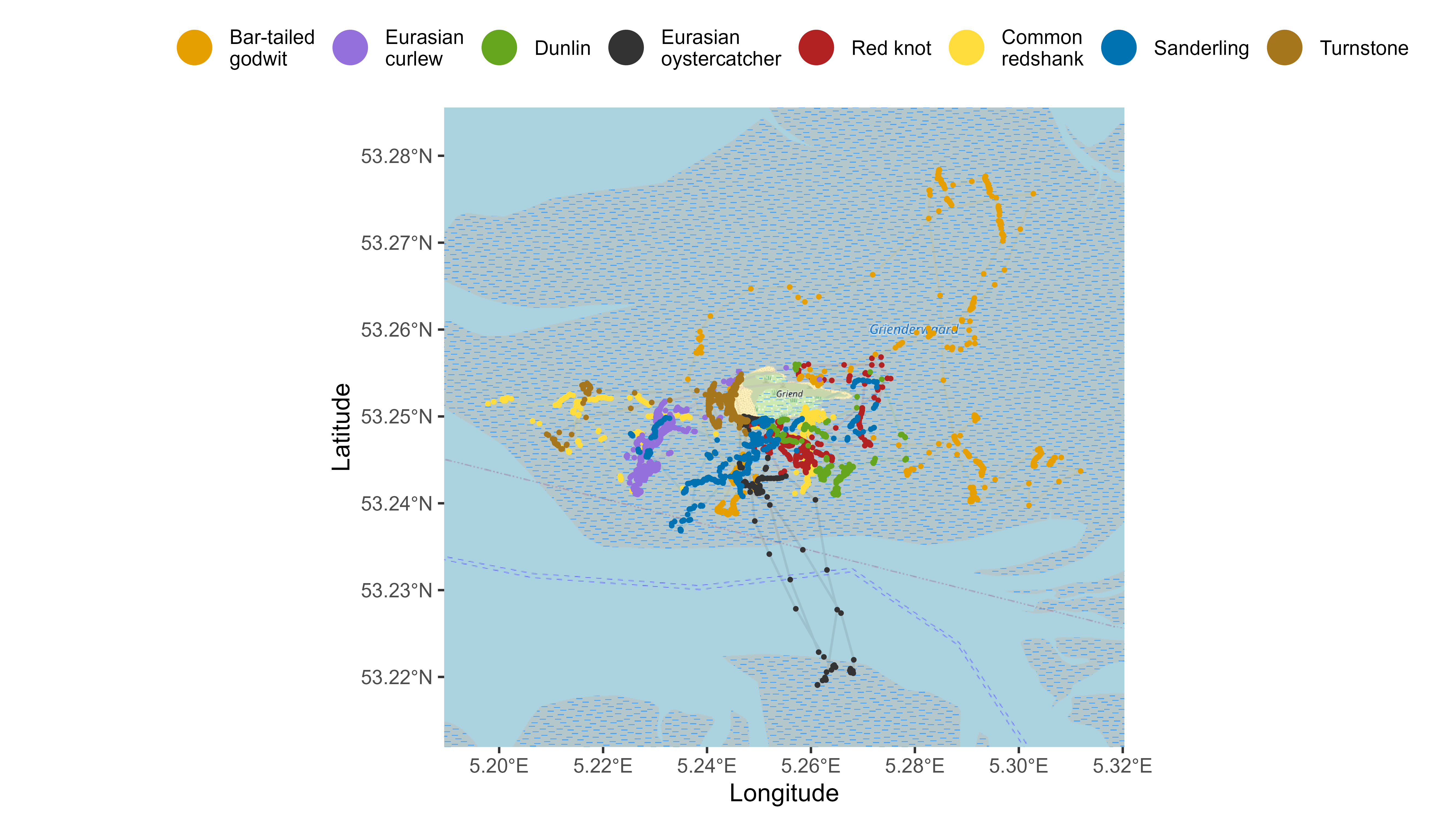
Static map with satellite image
Base R map
Plot with simple base map
The plotting region can be extended by specifiying buffer (in meters), and the scale of the scalebar (in kilometers) can be adjusted. To inspect the localizations, color_by can be specified to colour the localizations by time since first localization in plot (“time”), standard deviation of the x- and y-coordinate (“sd”), or the number of base stations used for calculating the localization (“nbs”). By specifiying the full path and file name (with extension) in fullname, it is possible to save the plot as a .png. If necesarry, the legend can also be located elsewhere on the plot with Legend.
# Load example data
data <- data_example[tag == data_example[1, tag]]

# Transform to sf
d_sf <- atl_as_sf(data, additional_cols = names(data))

# Plot the tracking data with a simple background
atl_plot_tag(
  data = d_sf, tag = NULL, fullname = NULL, buffer = 1,
  color_by = "time"
)
## [1] "Ensure that data has the UTM 31N coordinate reference system."
# Note: function opens device and therefore the plot is not shown in markdownPlot with OpenStreetMap
With the function atl_plot_tag_osm() it is possible to
plot the track on a satellite image with the library OpenStreetMap. The
region of the the satellite image can be extended by specifying a buffer
(in meters) in the function atl_bbox The other options are similar to
atl_plot_tag (see earlier).
library(OpenStreetMap)
library(sf)

# Load example data
data <- data_example[tag == data_example[1, tag]]

# make data spatial and transform projection to WGS 84 (used in osm)
d_sf <- atl_as_sf(data, additional_cols = names(data))
d_sf <- sf::st_transform(d_sf, crs = sf::st_crs(4326))

# get bounding box
bbox <- atl_bbox(d_sf, buffer = 500)

# extract openstreetmap
# other 'type' options are "osm", "maptoolkit-topo", "bing", "stamen-toner",
# "stamen-watercolor", "esri", "esri-topo", "nps", "apple-iphoto", "skobbler";
map <- OpenStreetMap::openmap(c(bbox["ymax"], bbox["xmin"]),
  c(bbox["ymin"], bbox["xmax"]),
  type = "bing", mergeTiles = TRUE
)

# Plot the tracking data on the satellite image
atl_plot_tag_osm(
  data = d_sf, tag = NULL, mapID = map, color_by = "time",
  fullname = NULL, scalebar = 3
)

# Note: function opens device and therefore the plot is not shown in markdown