Filter data

This vignette shows how to filter WATLAS-data based on spatial boundaries, temporal windows, and positioning errors.

Loading the data

In the previous step Load and check data, we have saved the raw data. You can run the code in sequence without saving the data, but extracting and processing large datasets can take a long time. Here, we work with the previously saved example data.

# packages
library(tools4watlas)
library(lubridate)
library(sf)
library(ggplot2)
library(scales)
library(viridis)

# path to csv with raw data
data_path <- system.file(
  "extdata", "watlas_data_raw.csv",
  package = "tools4watlas"
)

# load data
data <- fread(data_path, yaml = TRUE)

Spatial filtering

Sometimes it can make sense to subset data for a particular area of interest, or for outliers (i.e. positions outside the tracking region). In this example, we subset all data around Griend, Richel and Ballastplaat and exclude the rest. Note that in this example all example data fall within the specified bounding box, so no data will be filtered out.

# start with a location central to the area of interest
griend_east <- st_sfc(st_point(c(5.275, 53.2523)), crs = st_crs(4326)) |>
  st_transform(crs = st_crs(32631))

# create a bounding box around the location with a buffer
# that includes Griend, Richel and Ballastplaat
bbox <- atl_bbox(griend_east, asp = "16:9", buffer = 8000)
bbox_sf <- st_as_sfc(bbox)

## plot the data and bounding box

# create a base map for background
bm <- atl_create_bm(buffer = 10000) # default centre is Griend

# to speed-up plotting the tracking data, we will make a heatmap
# round tracking data to 1 ha (100x100 meter) grid cells
data[, c("x_round", "y_round") := list(
  plyr::round_any(x, 100),
  plyr::round_any(y, 100)
)]

# N by location
data_subset <- data[, .N, by = c("x_round", "y_round")]

# plot data with bounding box
bm +
  geom_tile(
    data = data_subset, aes(x_round, y_round, fill = N),
    linewidth = 0.1, show.legend = TRUE
  ) +
  geom_sf(data = bbox_sf, color = "firebrick", fill = NA) +
  scale_fill_viridis(
    option = "A", discrete = FALSE, trans = "log10", name = "N positions",
    breaks = trans_breaks("log10", function(x) 10^x),
    labels = trans_format("log10", math_format(10^.x)),
    direction = -1
  ) +
  # set extend again (overwritten by geom_sf) with 1 km buffer around bbox
  coord_sf(
    xlim = c(bbox["xmin"] - 1000, bbox["xmax"] + 1000),
    ylim = c(bbox["ymin"] - 1000, bbox["ymax"] + 1000), expand = FALSE
  )

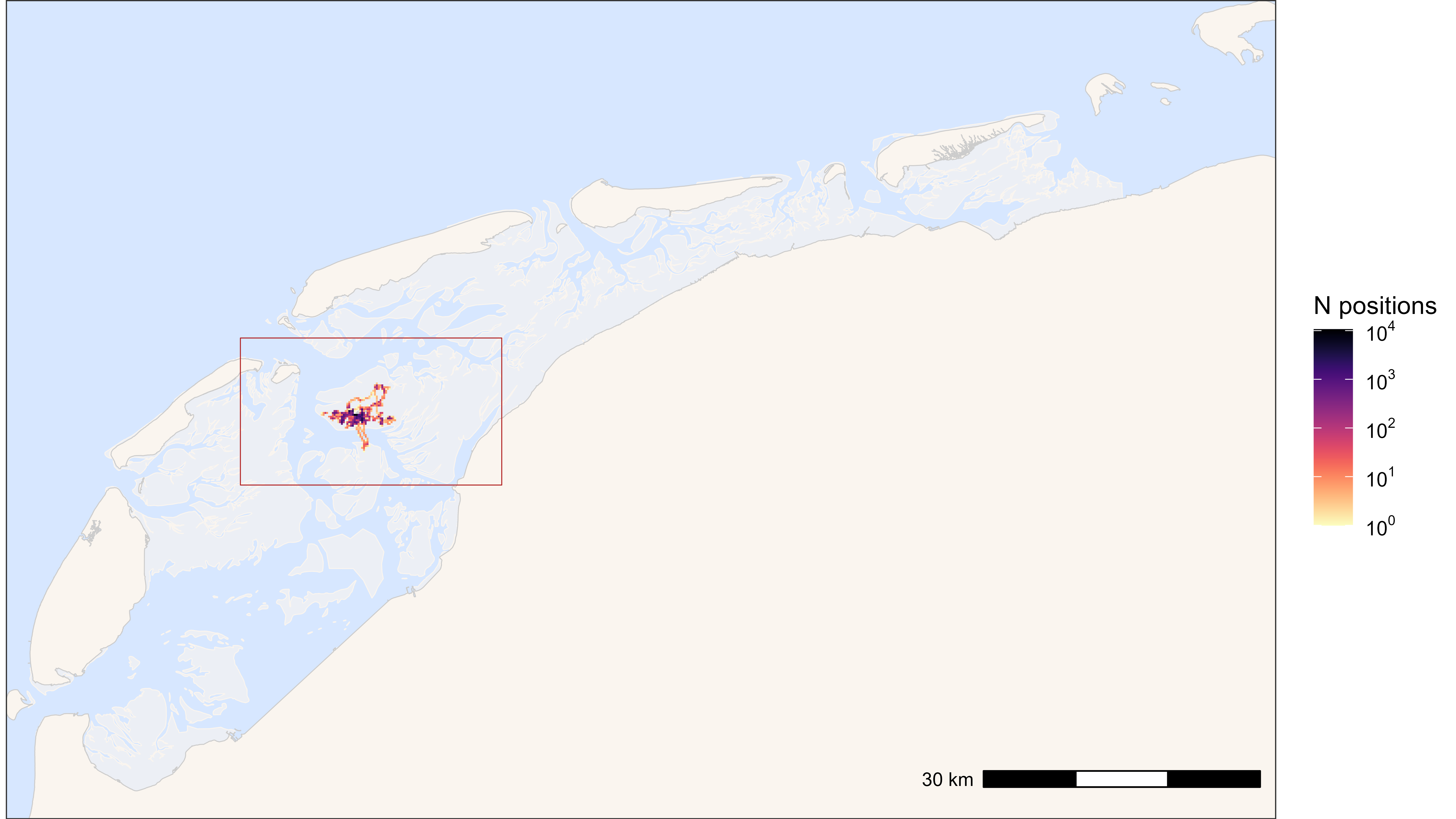
Heatmap of all positions with bounding box (red)

# remove rounded coordinates columns that were needed for making the heatmap
data[, c("x_round", "y_round") := NULL]

# filter data with bounding box
# note: when filtering with a rectangle bounding box
# and large datasets, using th range is faster than sf_polygon
data <- atl_filter_bounds(
  data = data,
  x = "x",
  y = "y",
  x_range = c(bbox["xmin"], bbox["xmax"]),
  y_range = c(bbox["ymin"], bbox["ymax"]),
  remove_inside = FALSE
)

If data are removed, one might first want to look at what was removed. This can be done like shown here (code not run as nothing was removed in our example).

# check what was removed
data_removed <- atl_filter_bounds(
  data = data,
  x = "x",
  y = "y",
  x_range = c(bbox["xmin"], bbox["xmax"]),
  y_range = c(bbox["ymin"], bbox["ymax"]),
  remove_inside = TRUE
)

# create a base map
bm <- atl_create_bm(data_removed, buffer = 1000)

# check removed data
bm +
  geom_point(
    data = data_removed, aes(x, y), color = "firebrick",
    size = 0.5, alpha = 1, show.legend = FALSE
  ) +
  geom_sf(data = bbox_sf, color = "firebrick", fill = NA) +
  # set extend again (overwritten by geom_sf) with 1 km buffer around bbox
  coord_sf(
    xlim = c(bbox["xmin"] - 1000, bbox["xmax"] + 1000),
    ylim = c(bbox["ymin"] - 1000, bbox["ymax"] + 1000), expand = FALSE
  )

On a finer level, depending on the analysis, one might want to assign all positions that are within a certain polygon. This can be done with atl_within_polygon(). In this example we assign a new column logic column with "on_grienderwaard to distinguish all positions on the mudflats around Griend.

# assign positions within the polygon of Grienderwaard
data <- atl_within_polygon(
  data, polygon = grienderwaard, col_name = "on_grienderwaard"
)

# new bounding box using Grienderwaard for plot
bbox <- atl_bbox(grienderwaard, buffer = 1500)

# plot points on and out of Grienderwaard
bm +
  geom_path(
    data = data, aes(x, y, colour = on_grienderwaard),
    linewidth = 0.5, alpha = 0.1, show.legend = TRUE
  ) +
  geom_point(
    data = data, aes(x, y, colour = on_grienderwaard),
    size = 0.5, alpha = 1, show.legend = TRUE
  ) +
  scale_color_discrete() +
  theme(legend.position = "top") +
  # add Grienderwaard polygon
  geom_sf(data = grienderwaard, color = "firebrick", fill = NA) +
  # set extend again (overwritten by geom_sf)
  coord_sf(
    xlim = c(bbox["xmin"], bbox["xmax"]),
    ylim = c(bbox["ymin"], bbox["ymax"]), expand = FALSE
  )

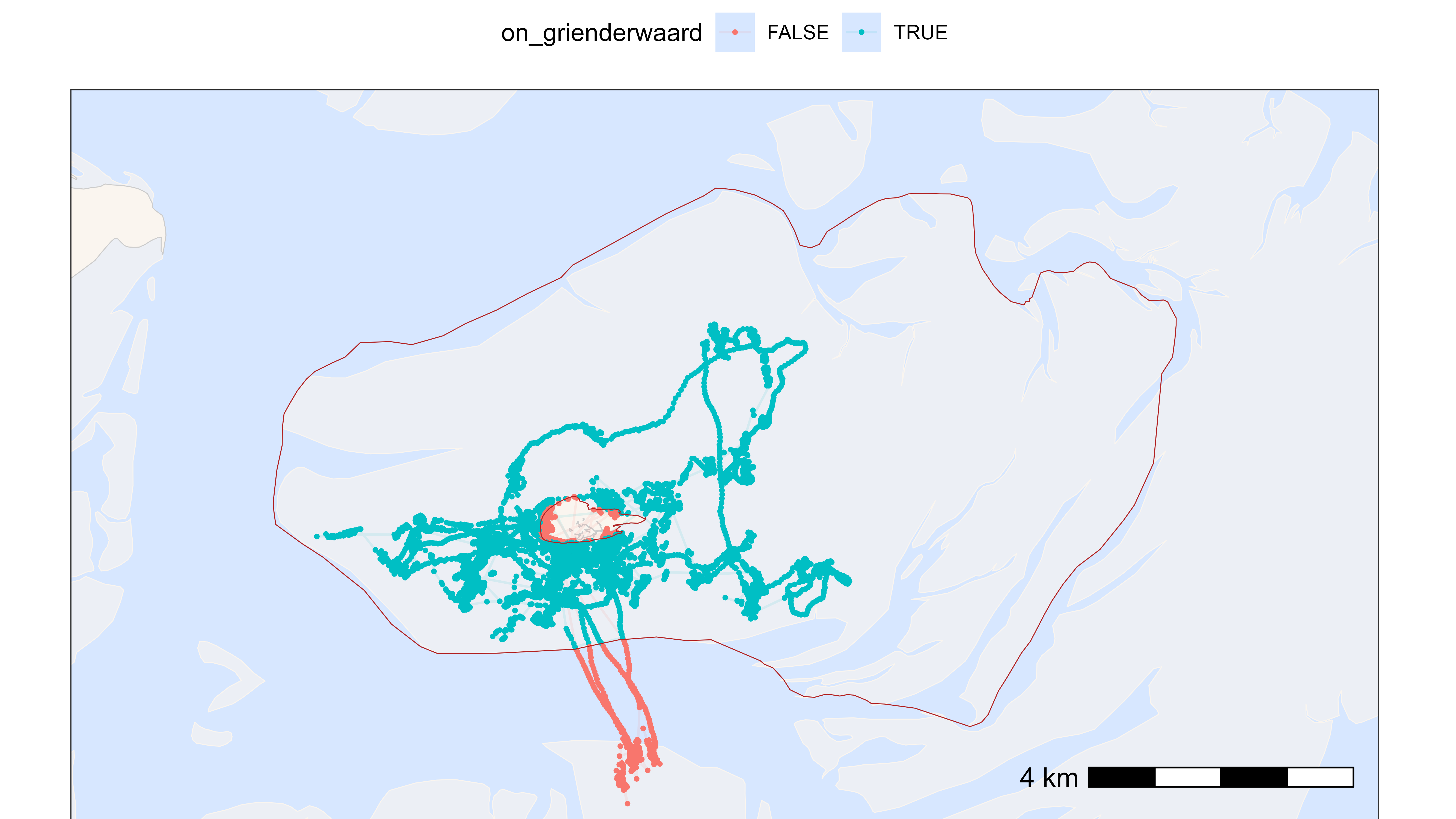
Plot with positions within and outside of Grienderwaard

Temporal filtering

Here, we show examples of filtering the data by timestamp. Because the birds need to adjust after being caught and fitted with a tag, we exclude the first 24 hours after release. Similarly, we can exclude positions at the end, e.g. after the tag fell off, or the bird died, etc. To identify such circumstances, it can be helpful to plot the last 1,000 positions for each tag (see vignette: plotting data).

Some tagged birds might not provide a lot of data, for instance, because they left the study area directly after release. For robust analyses, it might therefore be useful to exclude birds with few data. Below, we will exclude tags with less than 100 positions, but note that none of the birds in the example data is actually filtered out.

# load meta data
all_tags_path <- system.file(
  "extdata", "tags_watlas_subset.xlsx", package = "tools4watlas"
)
all_tags <- readxl::read_excel(all_tags_path, sheet = "tags_watlas_all") |>
  data.table()

# specify the time zone as CET, and standardise to UTC
all_tags[, release_ts := force_tz(as_datetime(release_ts), tzone = "CET")]
all_tags[, release_ts := with_tz(release_ts, tzone = "UTC")]

# join data tables
all_tags[, tag := as.character(tag)]
data[all_tags, on = "tag", `:=`(release_ts = i.release_ts)]

# exclude positions before the release with an additional 24h
data <- data[datetime > release_ts + 24 * 3600]

# exclude positions after a specific date (e.g. when the bird died):
data <- data[!(tag == "3103" &
                 datetime > as.POSIXct("2023-09-25 15:00:00", tz = "UTC"))]

# exclude tags with less than 100 positions
data[, N := .N, tag]
data[N < 100] |> unique(by = "tag")
data <- data[N > 100]

# clean up data table by removing unneeded columns
data[, release_ts := NULL]
data[, N := NULL]

Filtering location errors

Here, we will show two ways of filtering the data by positioning errors. First, by the size of the error estimate as provided by the algorithm for calculating positions. Second, based on unreleastic speeds between sequential positions.

Based on WATLAS error estimate

The position estimates come with three variance estimates: varx, vary and covarxy (see data explanation). Depending on the goal of the study, one can choose different variance thresholds. If its important that the position data is accurate, the value can be set low at e.g. 2,000 (see appendix S1 panel A in Beardsworth et al. 2022). Another strategy is to have a higher, less conservative threshold (e.g. 5,000) and use the resulting larger data volume to increase the quality by median smoothing.

# filter on the variance of the estimated X- and Y-coordinates
var_max <- 5000 # in meters squared

data <- atl_filter_covariates(
  data = data,
  filters = c(
    sprintf("varx < %s", var_max),
    sprintf("vary < %s", var_max)
  )
)

## Note: 0.54% of the dataset was filtered out, corresponding to 470 positions.

Based on speed

A bird’s speed can be calculated from sequential positions and used for filtering unrealistic high speeds. This is straightforward for positions with very high speeds between itself and the positions before and after (the so-called incoming and outgoing speed, respectively). See Gupte et al. 2022 for more background.

To choose a maximum speed threshold, it is important to plot the distribution of speed and best also the tracks around the outliers using atl_check_tag(highlight_outliers = TRUE). We found that its better to have a large maximum speed threshold and only filter out extreme speeds. Remaining erroneous positions can be filter out by smoothing the data (e.g. by median smoothing).

# calculate speed
data <- atl_get_speed(data, type = c("in", "out"))

# plot speed (subset relevant range)
ggplot(data = data[!is.na(speed_in) & speed_in > 5 & speed_in < 100]) +
  geom_histogram(aes(x = speed_in), bins = 50) +
  labs(x = "Speed in (m/s)") +
  theme_bw()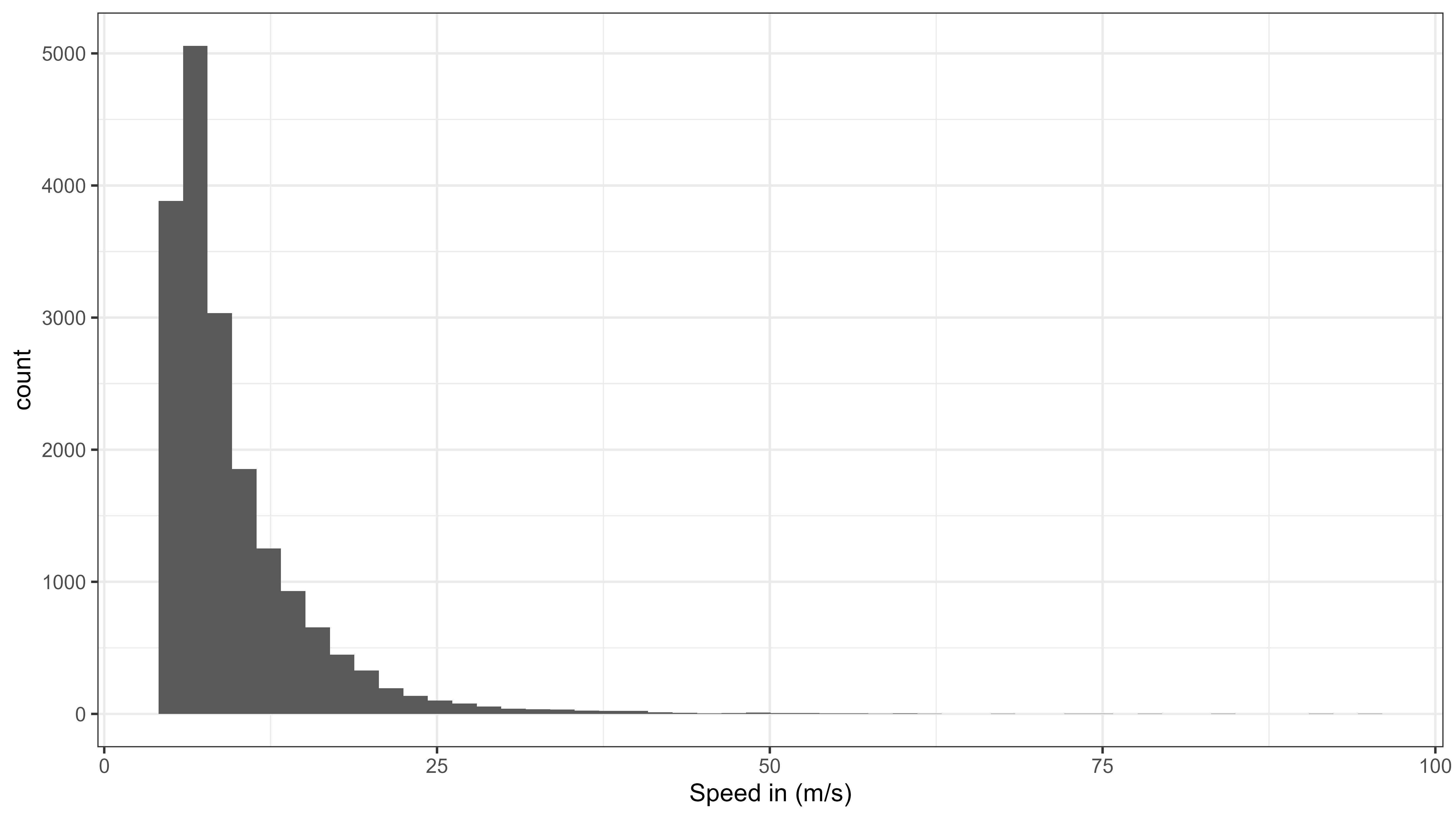

Histogram of speed moved from all data

# filter by speed
speed_max <- 35 # m/s (126 km/h)

data <- atl_filter_covariates(
  data = data,
  filters = c(
    sprintf("speed_in < %s | is.na(speed_in)", speed_max),
    sprintf("speed_out < %s | is.na(speed_out)", speed_max)
  )
)

## Note: 0.36% of the dataset was filtered out, corresponding to 315 positions.

# recalculate speed
data <- atl_get_speed(data, type = c("in", "out"))

Save the filtered data for the next steps

# save data
fwrite(data, file = "../inst/extdata/watlas_data_filtered.csv", yaml = TRUE)