Smooth and thin data

This vignette shows how to smooth and thin WATLAS data.

# Packages
library(tools4watlas)
library(data.table)
library(ggplot2)

# Path to csv with raw data
data_path <- system.file(
  "extdata", "watlas_data_filtered.csv",
  package = "tools4watlas"
)

# Load data
data <- fread(data_path, yaml = TRUE)

Median smooth data

To further reduce error in the localization data, a basic smoother such as a median filter can be applied. The resulting table has the smoothed location stored in the x and y column and the original location stored in the x_raw and y_raw column.

# Smooth the data
data <- atl_median_smooth(data, moving_window = 5)

Recalculate speed

After smoothing the data, the speeds need to be recalculated. We now also calculate turning angles. Note: the distance between smoothed positions can be 0 and therefore will produce NAs and a warning

# Recalculate speed
data <- atl_get_speed(data, type = c("in", "out"))

Look at the data

This plot just shows one example.

# subset first tag
data_subset <- data[tag == data[1]$tag]

# subset some data to look at
from <- min(data_subset[, datetime]) + 1 * 3600
to <- min(data_subset[, datetime]) + 12 * 3600
data_subset <- data_subset[datetime %between% c(from, to)]

# Create basemap
bm <- atl_create_bm(data_subset)

# Plot
bm +
  geom_path(
    data = data_subset, aes(x_raw, y_raw),
    color = "firebrick3", linewidth = 0.5
  ) +
  geom_path(
    data = data_subset, aes(x, y),
    color = "black", linewidth = 0.5
  ) +
  geom_point(
    data = data_subset, aes(x_raw, y_raw),
    color = "firebrick3", size = 1.2
  ) +
  geom_point(
    data = data_subset, aes(x, y),
    color = "black", size = 1
  )

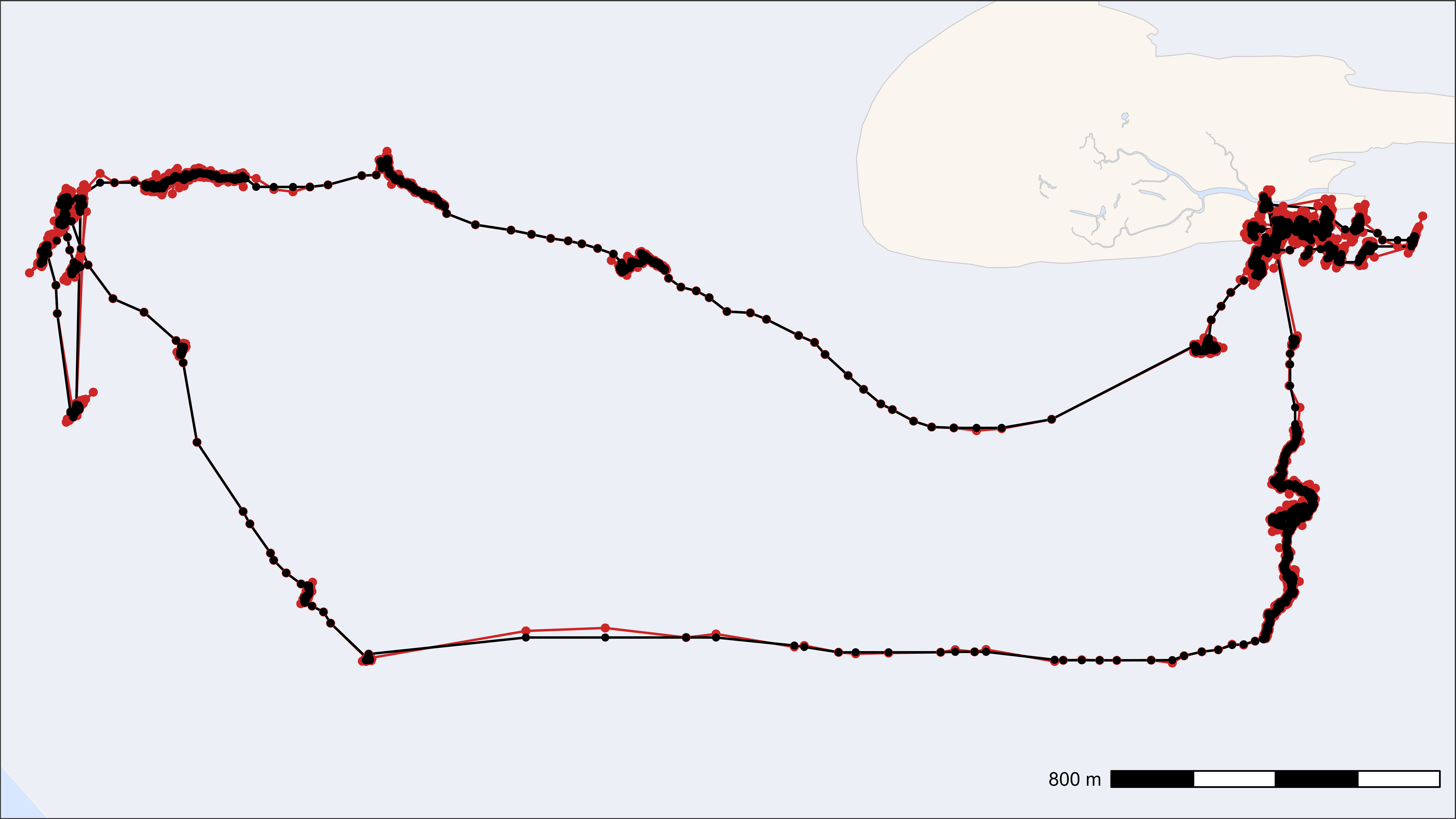
Smoothed track (black) on top of raw track (red)

Thin data

Depending on the desired analysis, it might make sense to thin data, either by aggregation or by subsampling. Both methods return fixed time steps (depending on the interval).

By aggregation

Returns the average of all columns for each time step. The additional column n_aggregated shows how many locations were aggregated for this location. Time and datetime are returned rounded to the interval.

# Thin the data by aggregation with a 60-second interval
thinned_aggregated <- atl_thin_data(
  data = data,
  interval = 60,
  id_columns = "tag",
  method = "aggregate"
)

# Show head of selected data
head(thinned_aggregated[, .(tag, time, datetime, x, y, n_aggregated)]) |>
  knitr::kable(digits = 2)

tag	time	datetime	x	y	n_aggregated
3027	1695438780	2023-09-23 03:13:00	650705.6	5902556	3
3027	1695439140	2023-09-23 03:19:00	650722.1	5902562	4
3027	1695439200	2023-09-23 03:20:00	650712.0	5902563	10
3027	1695439260	2023-09-23 03:21:00	650702.9	5902562	1
3027	1695439440	2023-09-23 03:24:00	650705.2	5902576	6
3027	1695439500	2023-09-23 03:25:00	650700.1	5902562	17

By subsampling

Returns one random location for each time step. The additional column n_subsampled shows from how many locations this location was sampled.

# Thin the data by subsampling with a 60-second interval
thinned_subsampled <- atl_thin_data(
  data = data,
  interval = 60,
  id_columns = "tag",
  method = "subsample"
)

# Show head of selected data
head(thinned_subsampled[, .(tag, time, datetime, x, y, n_subsampled)]) |>
  knitr::kable(digits = 2)

tag	time	datetime	x	y	n_subsampled
3027	1695438802	2023-09-23 03:13:22	650705.6	5902556	3
3027	1695439189	2023-09-23 03:19:49	650721.0	5902559	4
3027	1695439201	2023-09-23 03:20:01	650723.1	5902564	10
3027	1695439261	2023-09-23 03:21:01	650702.9	5902562	1
3027	1695439477	2023-09-23 03:24:37	650702.8	5902562	6
3027	1695439501	2023-09-23 03:25:01	650709.9	5902598	17

Save data

# Save data
fwrite(thinned_aggregated,
  file = "../inst/extdata/watlas_data_aggregated.csv", yaml = TRUE
)