Create a basemap

This article shows how to make different basemaps for plotting movement data. We present three options for creating a basemap using: 1) polygons delineating areas of mudflat, water and land provided within the package (see also the Article Basemap data), 2) bathymetry data, 3) backgrounds from the package maptiles, and 4) the package OpenStreetMap.

Load packages

# packages
library(tools4watlas)
library(ggplot2)

Using polygons

One can create a simple basemaps of the study area by using the function atl_create_bm(). This function uses a data.table with x- and y-coordinates to check the required bounding box (which can be extended with a buffer in meters) and spatial features (polygons) of land, lakes, mudflats and rivers. Without adding spatial data, it will default to the spatial data provided in the package. By changing asp the desired aspect ratio can be chosen (default is “16:9”). The resulting map is always in EPSG:32631 (WGS 84 / UTM zone 31N), but the data can be provided in other projections, which then needs to be specified as projection.

Basemap with extent of movement data

Instead of using a priori coordinates to construct a basemap, one can also use the movement data to set the extent of the map.

# load example data
data <- data_example

# create basemap
bm <- atl_create_bm(data, buffer = 1000)

# plot
bm +
  geom_point(data = data, aes(x, y), alpha = 0.1, color = "darkorange")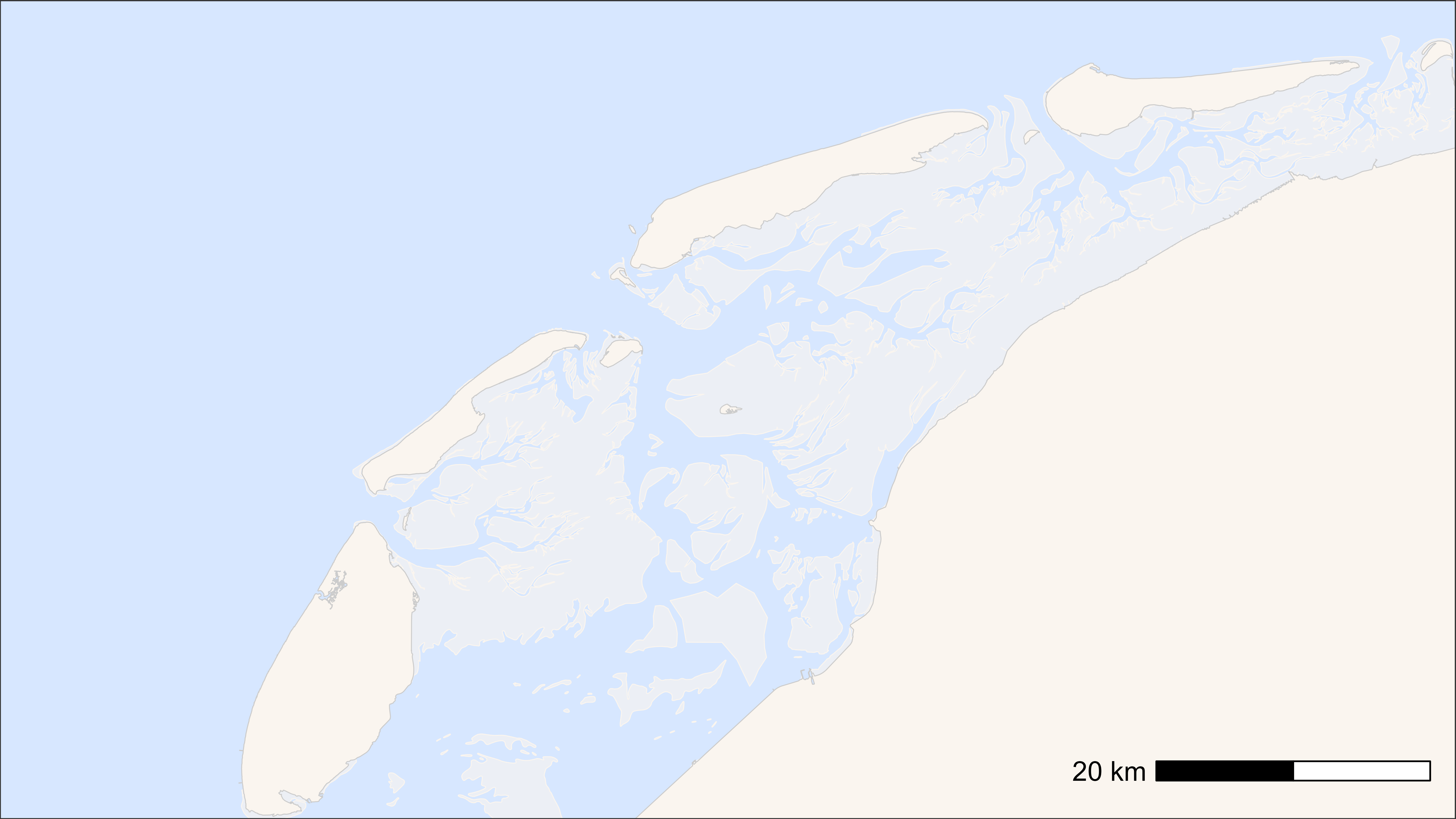

Basemap independent of movement data

This can be useful when one wants to zoom into a specific area of the plot or has an area of interest, but the movement data can extent beyond this specifieds range. If no data are provided, the function defaults to a map around Griend (our main study site) with a specified buffer.

# create basemap
bm <- atl_create_bm(buffer = 30000)

# plot
bm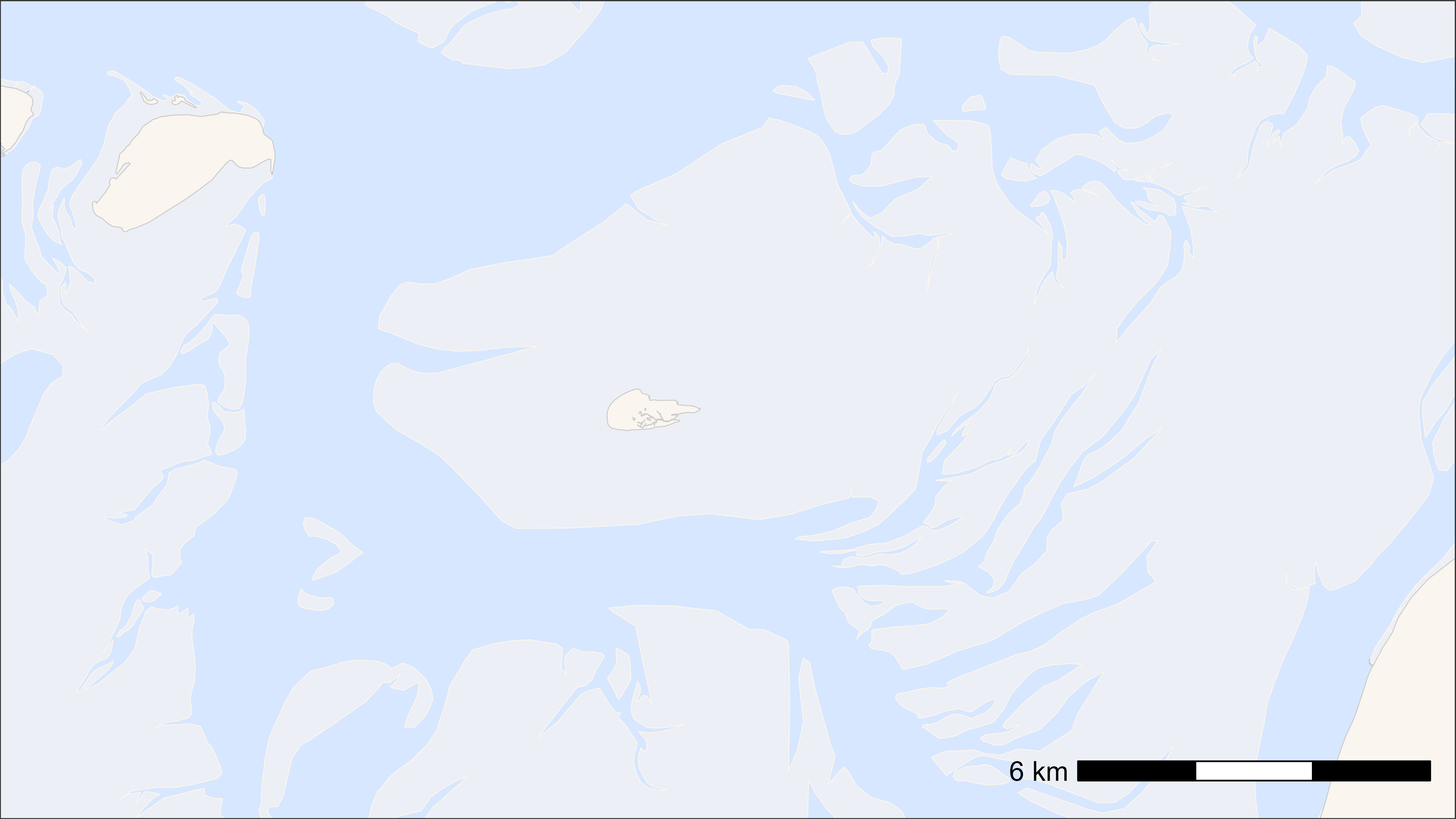

Alternatively, one can provide a table with one or multiple locations, which will then be used to make the map. This can for example be a location in EPSG:4326 (WGS 84 in degrees) that can be extracted from Google Maps by a right click on a specific location. Here I choose a point a bit east of Griend, to include Richel and Ballastplaat in the map.

# define location
location <- data.table(x = c(5.275), y = c(53.2523))

# create basemap
bm <- atl_create_bm(location, buffer = 7000, projection = sf::st_crs(4326))

# plot
bm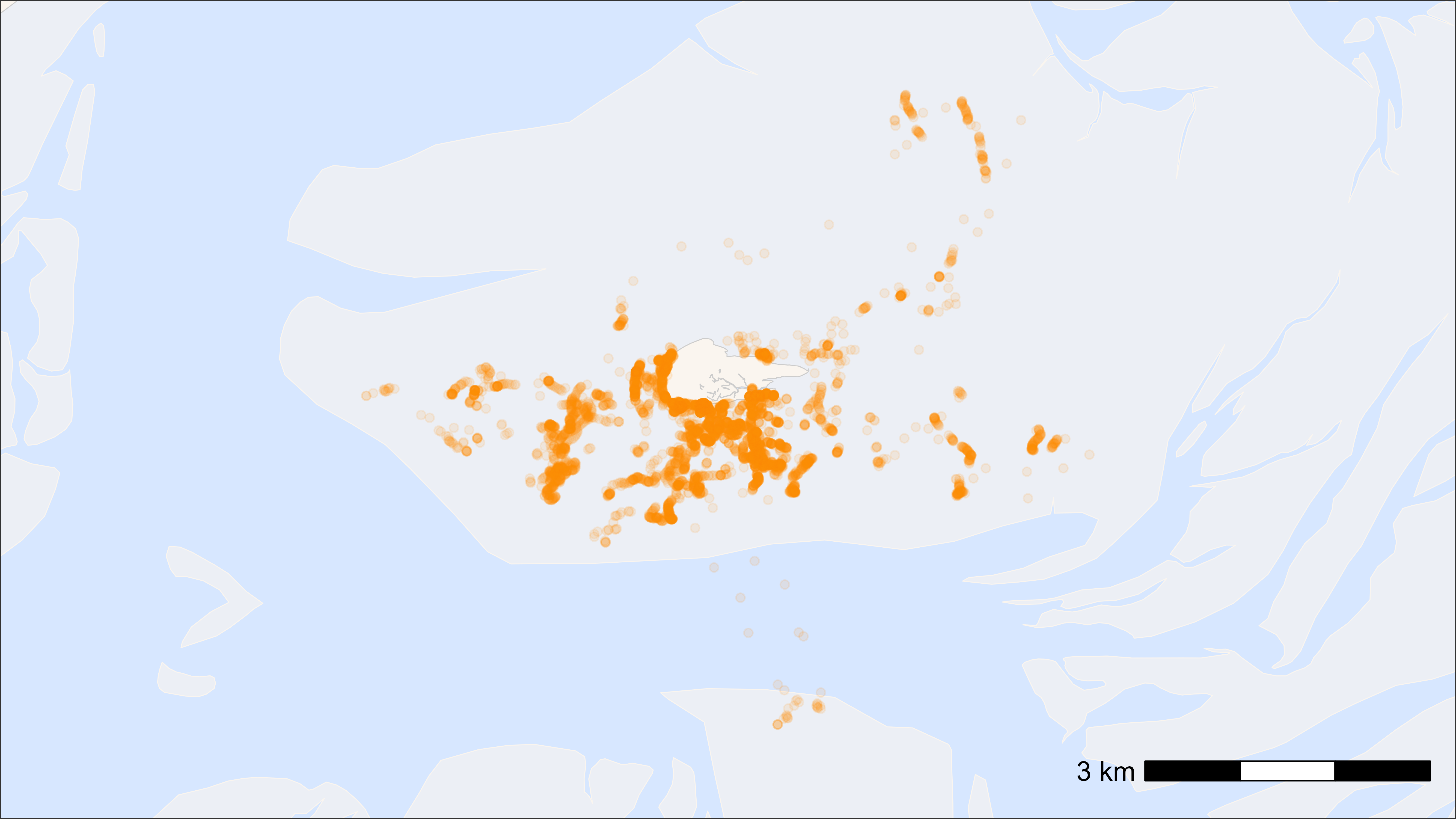

Instead of using one central point and a buffer we can also provide two points (corners of a rectangle) to specify the basemap. When we do this, we also might not want to use a buffer and a specific aspect ratio, so we can set buffer = 0 and asp = NULL, but if desired we can also use a buffer and an aspect ratio. The example below shows how to create a basemap around Griend and Richel with two corner points, which is useful when we want to zoom into a specific area of the map. The first point is north-west of Richel and the second point south-east of Griend.

# specify corner points
corner_points <- data.table(x = c(5.107, 5.330), y = c(53.303, 53.230))

# create basemap
bm <- atl_create_bm(
  corner_points,
  buffer = 0, asp = NULL, projection = sf::st_crs(4326)
)

# plot
bm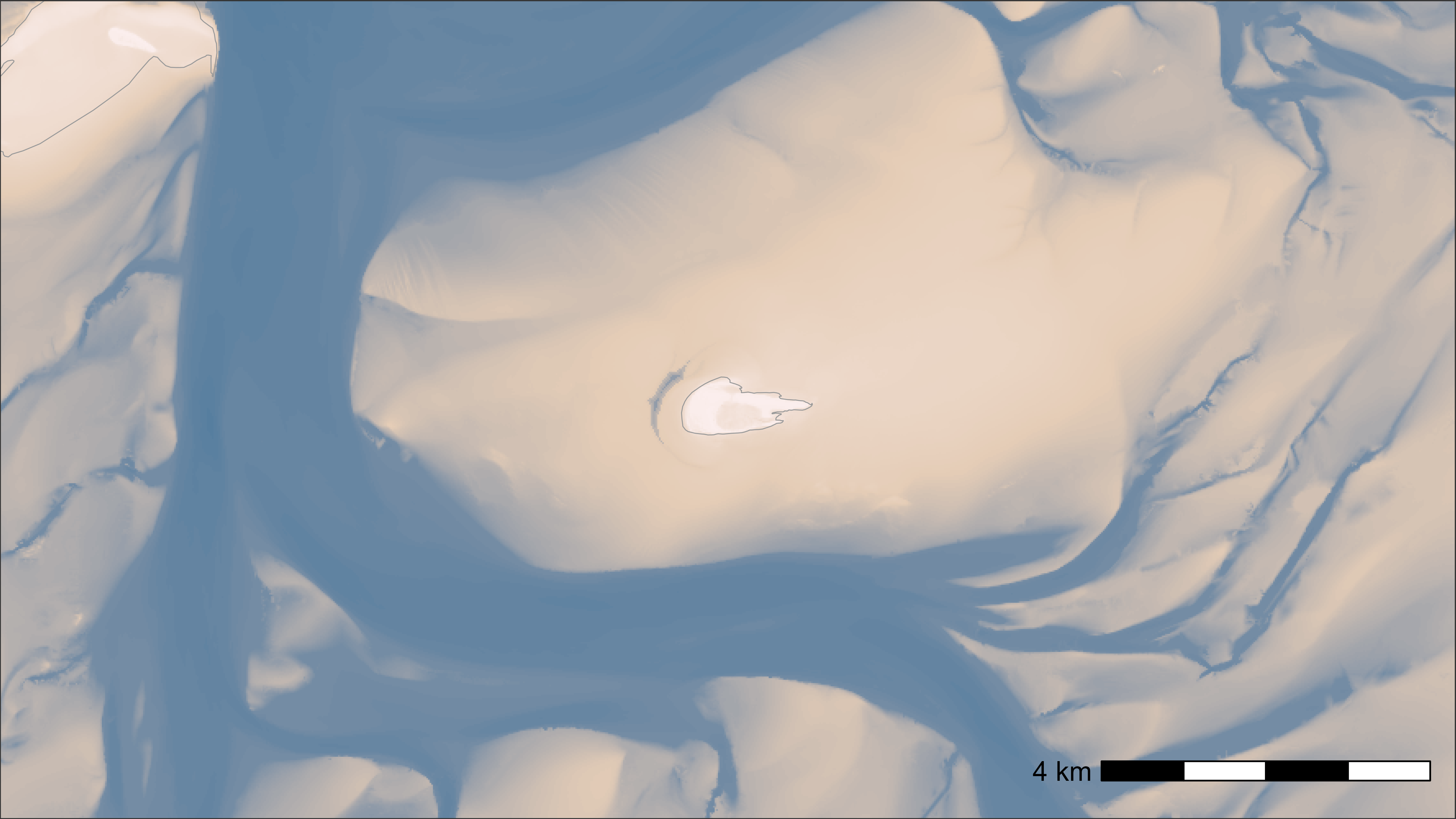

Using bathymetry data

Here, we use a raster file with bathymetry to construct a basemap. Bathymetry data can be found in the “Birds, fish ’n chips” SharePoint folder: Documents/data/GIS/rasters/. To run the script set the file path (fp) to the local copy of the folder on your computer. The data can also be downloaded from the Waddenregister.

# additional packages
library(terra)

# file path to Birds, fish 'n chips GIS/rasters folder
fp <- atl_file_path("rasters")

# load bathymetry data
bat <- rast(paste0(fp, "bathymetry/2024/bodemhoogte_20mtr_UTM31_int.tif"))

# create base map with bathymetry data
bm <- atl_create_bm(
  buffer = 5000, raster_data = bat, option = "bathymetry"
)

# plot
bm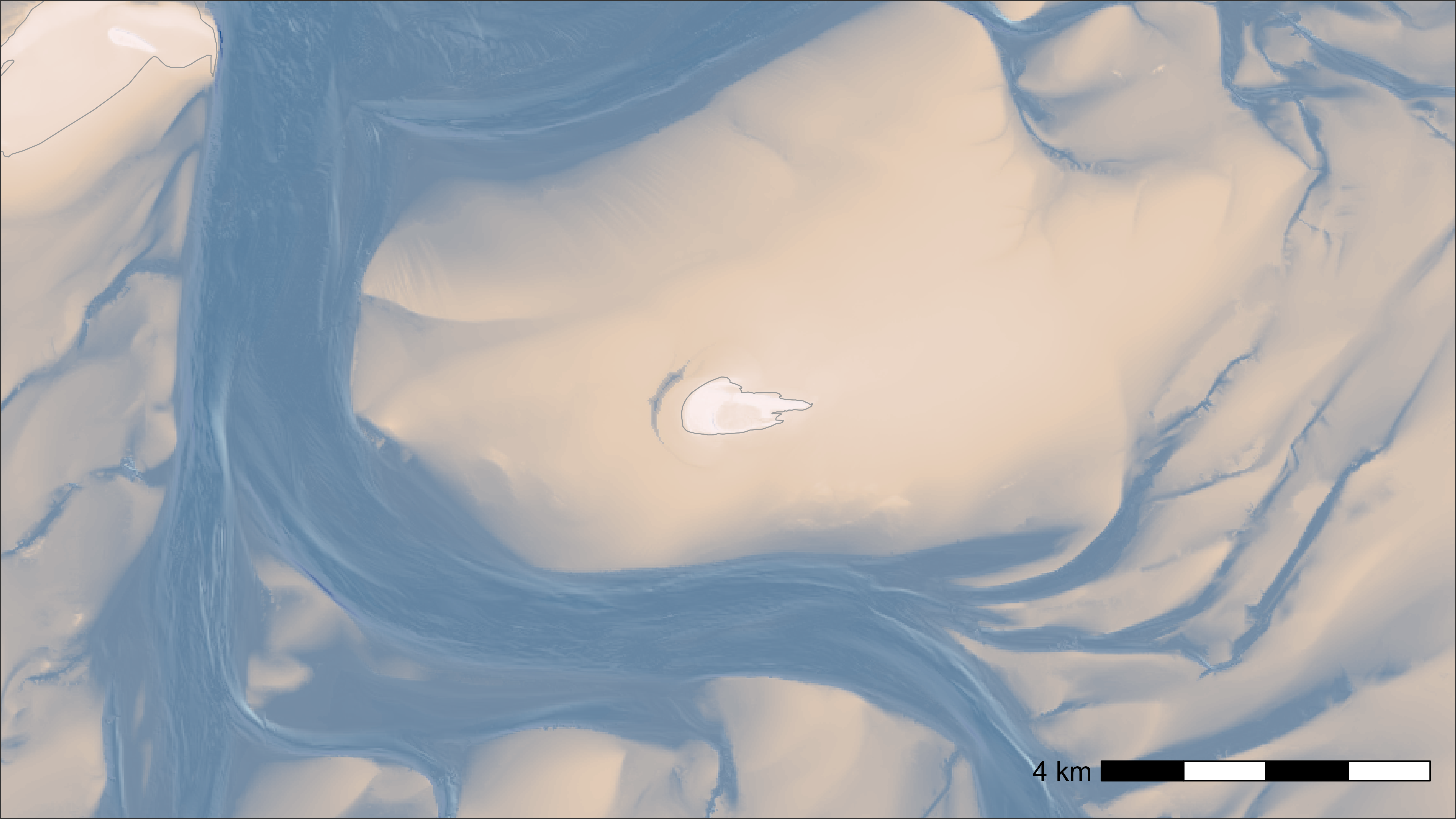

We can also add some shading (shade = TRUE) to the bathymetry data to highlight the geomorphological structures better. Note that calculating shading can take a while, especially for large maps. We remommend using this option only for polished maps.

# additional packages
library(terra)

# file path to Birds, fish 'n chips GIS/rasters folder
fp <- atl_file_path("rasters")

# load bathymetry data
bat <- rast(paste0(fp, "bathymetry/2024/bodemhoogte_20mtr_UTM31_int.tif"))

# create base map with bathymetry data
bm <- atl_create_bm(
  buffer = 5000, raster_data = bat, option = "bathymetry", shade = TRUE
)

# plot
bm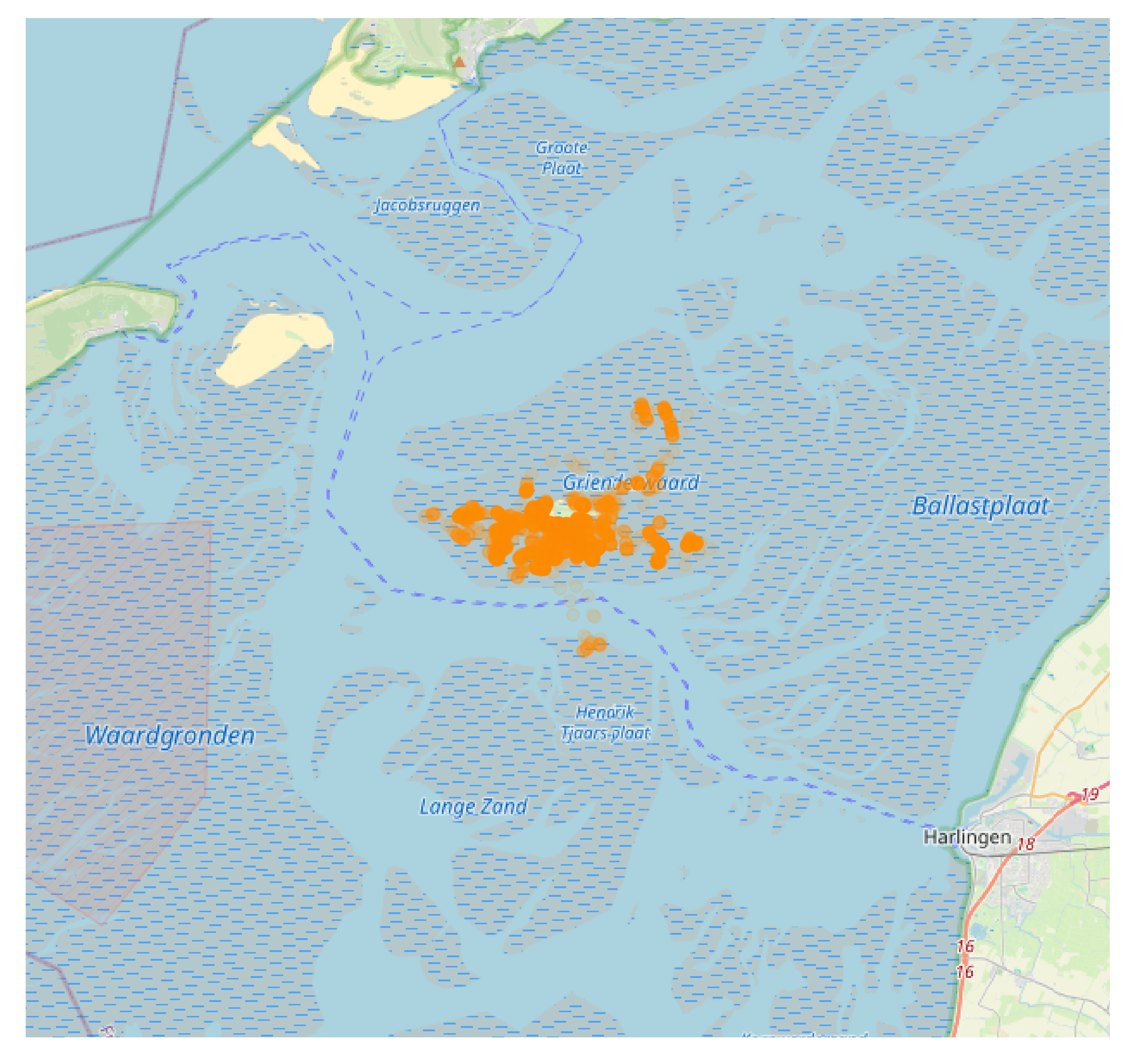

Using maptiles

The package maptiles provides an easy way to create basemaps from different tile providers (e.g., OpenStreetMap, Esri satellite images, Stamen toner, etc.). The function atl_create_bm_tiles() wraps around the maptiles functions to create a basemap based on movement data or specified bounding boxes and otherwise works like atl_create_bm(). It is best to use the standard EPSG:32631 (WGS 84 / UTM zone 31N) to create a bounding box (since this means the data don’t need to be transformed internally), but other projections also work. The output maps are, however, always in EPSG:4326, so movement data need to be transformed to be added to the plot. atl_transform_dt() can be used to add transformed positions to the data table.

Use satellite map

# satellite map and buffer around Griend
bm <- atl_create_bm_tiles(
  buffer = 15000, option = "Esri.WorldImagery", zoom = 12
)

# plot
bm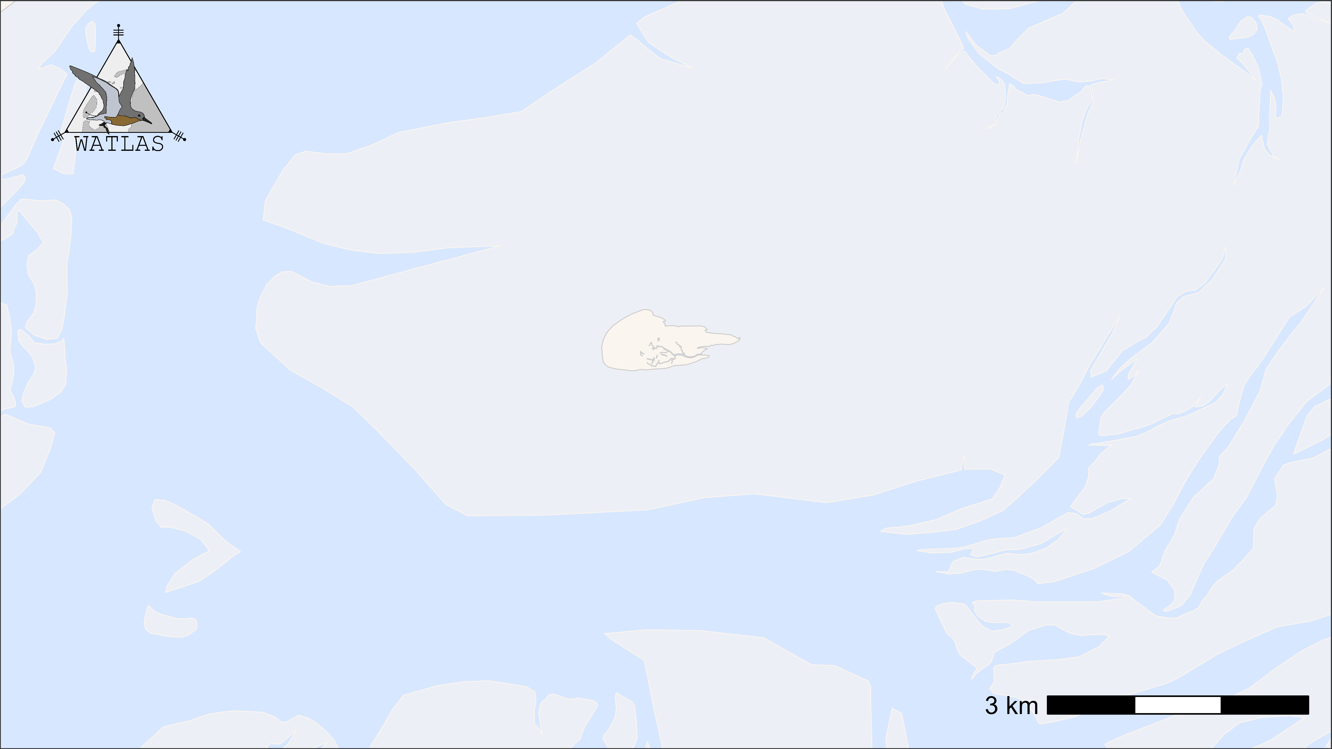

# example with bbox and adding movement data
data <- data_example

# add transformed coordinates in projection of the base map (EPSG:4326)
data <- atl_transform_dt(data)

# plot points and tracks using transformed coordinates.
bm +
  geom_path(
    data = data, aes(x_4326, y_4326, colour = tag),
    linewidth = 0.5, alpha = 0.1, show.legend = FALSE
  ) +
  geom_point(
    data = data, aes(x_4326, y_4326, colour = tag),
    size = 0.5, alpha = 1, show.legend = FALSE
  ) +
  scale_color_discrete(name = paste("N = ", length(unique(data$tag)))) +
  theme(legend.position = "top")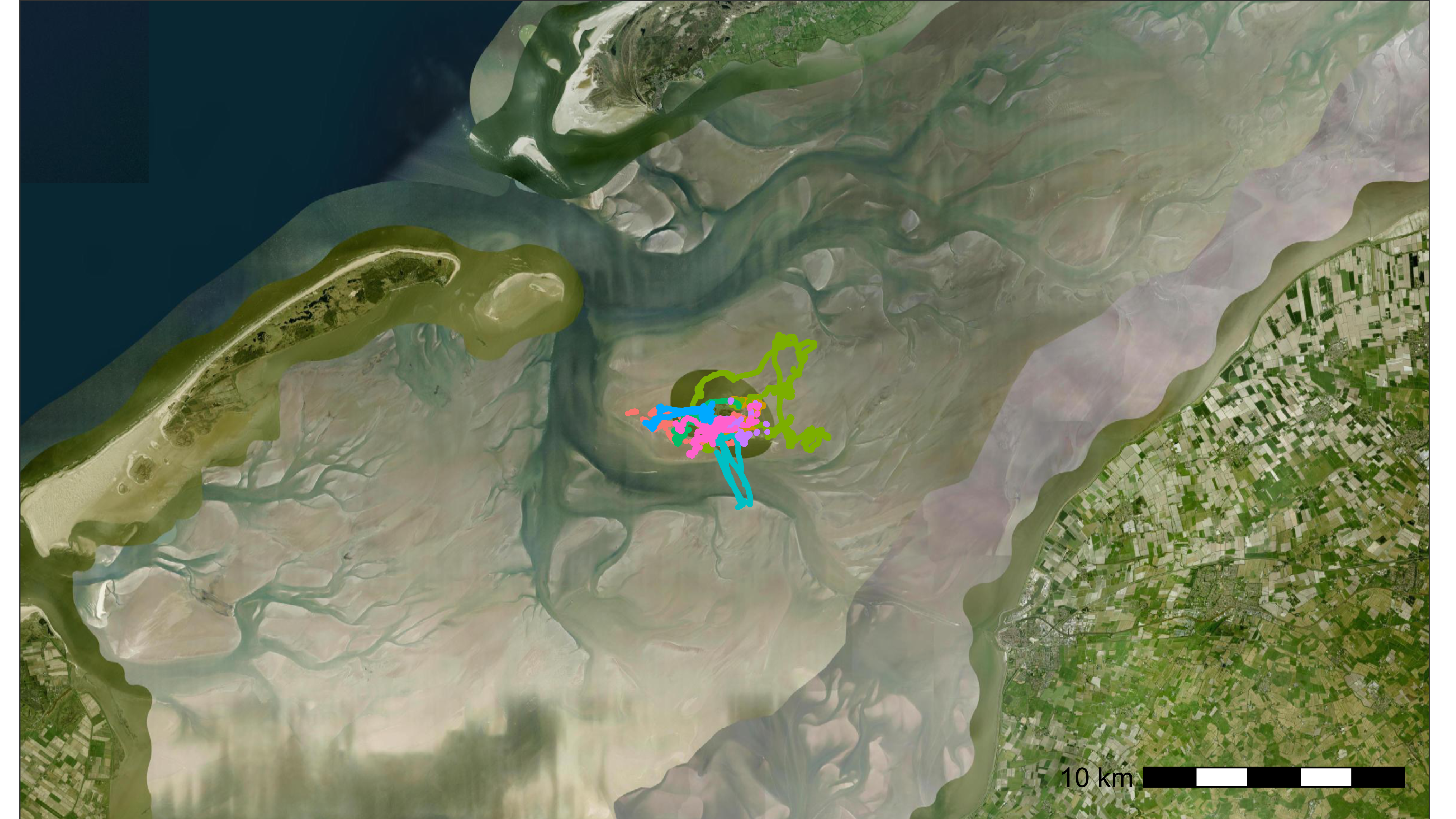

Using OpenStreetMap

A range of basemap options are provided by OpenStreetMap. First, we have to transform the data to WGS 84 to extract the basemap with the bounding box, and then transform our data to a Mercator projection to plot the data on top of the map.

Unfortunately, the type = "bing" (satellite image) is unstable and does not always work.

# additional packages
library(OpenStreetMap)
library(sf)

# load example data
data <- data_example

# make data spatial and transform projection to WGS 84 (used in osm)
d_sf <- atl_as_sf(data, additional_cols = c("tag", "datetime"))
d_sf <- st_transform(d_sf, crs = st_crs(4326))

# get bounding box
bbox <- atl_bbox(d_sf, asp = "16:9", buffer = 10000)

# extract openstreetmap
# other 'type' options are "osm", "maptoolkit-topo", "bing", "stamen-toner",
# "stamen-watercolor", "esri", "esri-topo", "nps", "apple-iphoto", "skobbler";
map <- openmap(
  c(bbox["ymax"], bbox["xmin"]),
  c(bbox["ymin"], bbox["xmax"]),
  type = "esri", mergeTiles = TRUE
)

bm <- autoplot.OpenStreetMap(map)

# transform points to Mercator and add transformed coordinates to data
d_sf <- st_transform(d_sf, crs = sf::st_crs(3857))
osm_coords <- st_coordinates(d_sf)
data[, `:=`(x_osm = osm_coords[, 1], y_osm = osm_coords[, 2])]

# plot
bm +
  geom_point(
    data = data, aes(x_osm, y_osm), alpha = 0.1, color = "darkorange"
  ) +
  coord_sf(crs = 3857, expand = FALSE) +
  theme(
    axis.title = element_blank(),
    axis.text = element_blank(),
    axis.ticks = element_blank(),
    panel.grid.major = element_blank(),
    panel.grid.minor = element_blank()
  )

Adding features to a map

Here, we show how to add additional features, like the WATLAS logo or receivers, to a map.

Add WATLAS logo

# additional packages
library(ggimage)

# load example data
data <- data_example

# create basemap
bm <- atl_create_bm(data, buffer = 1000)

# path to WATLAS logo
logo_path <- system.file(
  "extdata", "watlas_logo.png",
  package = "tools4watlas"
)

# define position based on data (here upper left corner)
# adjust as desired
x_pos <- min(data$x) - 2500
y_pos <- max(data$y)

# create table with image of the logo
di <- data.table(x = x_pos, y = y_pos, image = logo_path)

# plot basemap with logo
bm +
  geom_image(data = di, aes(x, y, image = image), size = 0.2)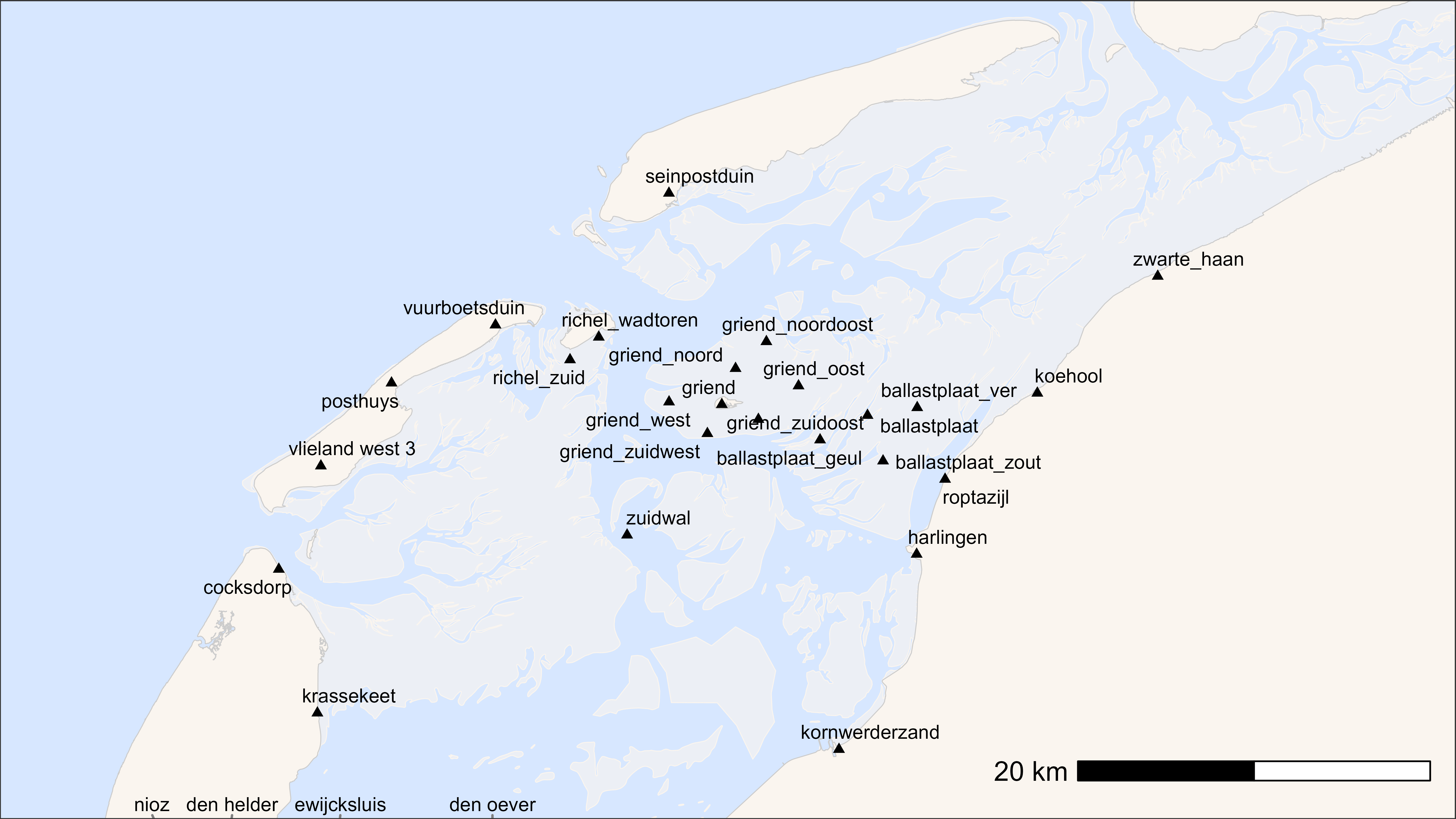

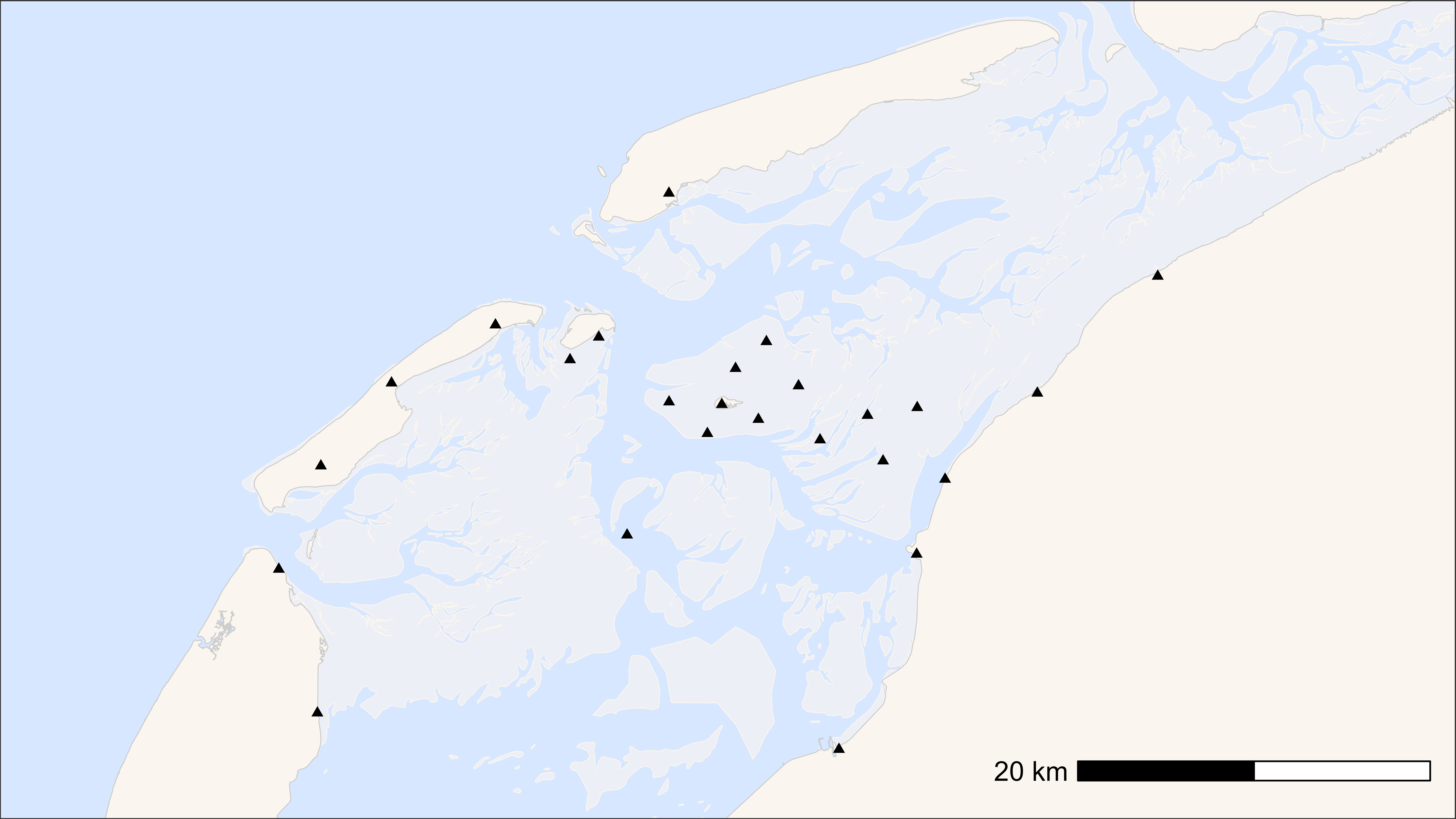
Add WATLAS receivers

Receiver data are managed by Allert. They are located in the “WATLAS” SharePoint folder: Documents/data/. Either specify the path to your local copy of this folder or add the path for your user in the atl_file_path() function.

# load example data
data <- data_example

# create basemap
bm <- atl_create_bm(data, buffer = 20000)

# file path to WATLAS teams data folder
fp <- atl_file_path("watlas_teams")

# load receivers data
dr <- readxl::read_excel(
  paste0(fp, "receivers/receiver specifications.xlsx"),
  sheet = "receivers"
) |>
  data.table()

# end date for active receivers as system date
dr[active == "ja", date_removed := as.POSIXct(Sys.time(), tz = "UTC")]

# subset all active in period of tracking data
start <- min(data$datetime)
end <- max(data$datetime)

# Check if each row includes period of tracking data
dr[, includes_data := (date_placed <= end & date_removed >= start)]
dr <- dr[includes_data == TRUE]

# plot basemap with receivers active during tracking period
bm +
  geom_point(data = dr, aes(x, y), pch = 17)

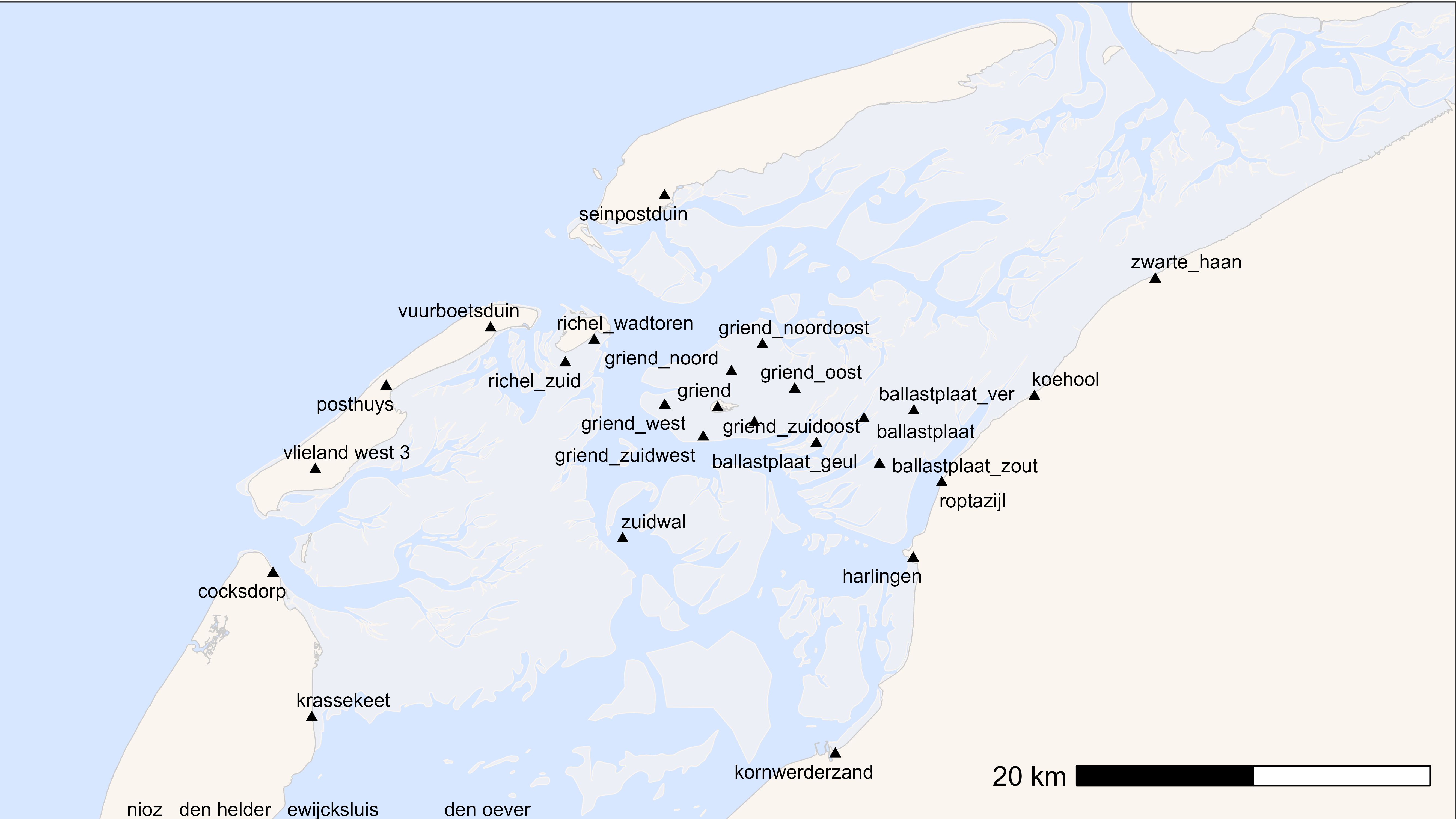
One can also add the name of the receiver.

# additional packages
library(ggrepel)

# plot basemap with receivers and label
bm +
  geom_point(data = dr, aes(x, y), pch = 17, size = 1.5) +
  geom_text_repel(
    data = dr, aes(x, y, label = location),
    max.overlaps = Inf,
    size = 3,
    point.padding = 0.5,
    segment.color = "grey50"
  )