Loading and checking data

Good to know

tools4watlas is based on data.table to be fast and efficient. A key feature of data.table is modification in place, where data is changed without making a copy. To prevent this (whenever it is not desired) use the function copy() to make a true copy of the data set.

# Packages
library(tools4watlas)
library(data.table)
library(ggplot2)
library(scales)
library(viridis)

Getting data

WATLAS data can either be loaded from a local SQLite database or a rem remote SQL database server. To do so, first select the tags and time period for which to extract data.

Use the tags_watlas_all.xlsx file (including metadata of all tags) or for collaborators the tags_watlas_subset.xlsx (including a subset of metadata) to select the desired tags. Here shown with the example data in tools4watlas.

Loading the tags_watlas_subset.xlsx will provide a table with the following columns:

Column	Description
season	Year in which the bird was caught
species	Species common name
tag	Tag ID with 4 digits
rings	Metal ring number
crc	Colour ring combo
release_ts	Release time stamp in CET
catch_location	Location where the bird was caught

Select the desired tags and time period

# Load meta data
all_tags_path <- system.file(
  "extdata", "tags_watlas_subset.xlsx", package = "tools4watlas"
)
all_tags <- readxl::read_excel(all_tags_path, sheet = "tags_watlas_all") |>
  data.table()

# Subset desired tags using data.table
# (For example all tags from season 2023)
tags <- all_tags[season == 2023]$tag

# Time period for which data should be extracted form the database (in CET)
from <- "2023-09-21 00:00:00"
to <- "2023-09-25 00:00:00"

Extract data from local SQLite file

First, the path and file name of the local SQLite database need to be provided. Then, with the established connection, the database can be queried for the selected tags and period. Here we will load the tagging data in one data.table.

# Database connection
sqlite_db <- system.file(
  "extdata", "watlas_example.SQLite", package = "tools4watlas"
)
con <- RSQLite::dbConnect(RSQLite::SQLite(), sqlite_db)

# Load data from database
data <- atl_get_data(
  tags,
  tracking_time_start = from,
  tracking_time_end = to,
  timezone = "CET",
  use_connection = con
)

# Close connection
RSQLite::dbDisconnect(con)

Alternatively, extract from remote SQL-database

To safely work with database credentials one option is to store them as environmental variables in R. This allows for example to have scripts on GitHub without sharing them. Restart R after adding variables to be able to access them. Ask Allert for the host, username and password and then add them in your environment like this:

# open .Renviron to edit
file.edit("~/.Renviron")

# add variables
host = "host"
username = "username"
password = "password"

# access variables (example)
Sys.getenv("variable_name")

atl_get_data does the same as when connecting to a local SQLite database when connecting to a remote database. In this example (chunk not run and only shown) we load the last three days of data from all tags of season 2024. Host, username and password are specified as environmental variables in this example, but can also be specified directly.

# Load meta data
all_tags_path <- "C:\\path\\tags_watlas_all.xlsx"
all_tags <- readxl::read_excel(all_tags_path, sheet = "tags_watlas_all") |>
  data.table()

# Subset all tags from 2024
tags <- all_tags[season == 2024]$tag

# Select N last days to get data from
days <- 3
from <- (Sys.time() - 86400 * days) |> as.character()
to <- (Sys.time() + 3600) |> as.character()

# Load data from database
data <- atl_get_data(
  tags,
  tracking_time_start = from,
  tracking_time_end = to,
  timezone = "CET",
  host = Sys.getenv("host"),
  database = "atlas2024",
  username = Sys.getenv("username"),
  password = Sys.getenv("password")
)

Data explanation

The resulting loaded WATLAS data will be a data.table with the following columns:

# Show head of the table
head(data) |> knitr::kable(digits = 2)

posID	tag	time	datetime	x	y	nbs	varx	vary	covxy
7914	3027	1695438802	2023-09-23 03:13:22	650692.8	5902549	3	46.97	392.42	126.62
7917	3027	1695438805	2023-09-23 03:13:25	650705.6	5902576	3	49.09	460.84	141.21
7921	3027	1695438808	2023-09-23 03:13:28	650691.6	5902536	3	58.18	471.81	155.89
8230	3027	1695439189	2023-09-23 03:19:49	650728.6	5902571	3	49.97	441.46	138.20
8234	3027	1695439192	2023-09-23 03:19:52	650721.0	5902556	3	5.34	28.16	8.58
8237	3027	1695439195	2023-09-23 03:19:55	650721.1	5902559	3	5.55	35.03	10.43

Column	Description
posID	Unique number for localizations
tag	4 digit tag number (character), i.e. last 4 digits of the full tag number
time	UNIX time (seconds)
datetime	Datetime in POSIXct (UTC)
x	X-cordinates in meters (UTM 31 N)
y	Y-cordinates in meters (UTM 31 N)
nbs	Number of Base Stations used in calculating coordinates
varx	Variance in estimating X-coordinates
vary	Variance in estimating Y-coordinates
covxy	Co-variance between X- and Y-coordinates

Save data

At this point it might be good to save the raw data, as extrating the data from the database can take a long time with big datasets. A convenient and fast way is to use fwrite from the data.table package. By including yaml = TRUE we make sure the data stays in the same format when we load it again. Change the file path when running this example.

# Save data
fwrite(data, file = "../inst/extdata/watlas_data_raw.csv", yaml = TRUE)

Check data

Data summary

Here we simply check for how many individuals we have data and how many positions by tag and date we have.

# Load data
data <- fread("../inst/extdata/watlas_data_raw.csv", yaml = TRUE)

# N individuals with tagging data
data[, .N, tag] |> nrow()

## [1] 8

# N positions, first and last data by tag ID
data[, .(
  N_positions = .N,
  fist_data = min(datetime),
  last_data = max(datetime)
), tag]

##       tag N_positions           fist_data           last_data
##    <char>       <int>              <POSc>              <POSc>
## 1:   3027       15859 2023-09-23 03:13:22 2023-09-23 22:24:26
## 2:   3038       15959 2023-09-23 00:00:01 2023-09-23 23:59:57
## 3:   3063       12614 2023-09-23 03:27:49 2023-09-23 22:24:55
## 4:   3100        8423 2023-09-23 04:21:46 2023-09-23 21:41:16
## 5:   3158       12533 2023-09-23 00:00:01 2023-09-23 23:59:57
## 6:   3188       10195 2023-09-23 00:00:45 2023-09-23 23:41:50
## 7:   3212        3856 2023-09-23 00:00:00 2023-09-23 23:59:56
## 8:   3288        8131 2023-09-23 00:00:03 2023-09-23 23:59:54

# add date
data[, date := as.Date(datetime)] |> invisible()

# N positions by species and day
data_subset <- data[, .N, by = .(tag, date)]

# Plot data
ggplot(data_subset, aes(x = date, y = tag, fill = N)) +
  geom_tile() +
  scale_fill_viridis(
    option = "A", discrete = FALSE, trans = "log10", name = "N positions",
    breaks = trans_breaks("log10", function(x) 10^x),
    labels = trans_format("log10", math_format(10^.x)),
    direction = -1
  ) +
  labs(x = "Date", y = "Tag") +
  theme_classic()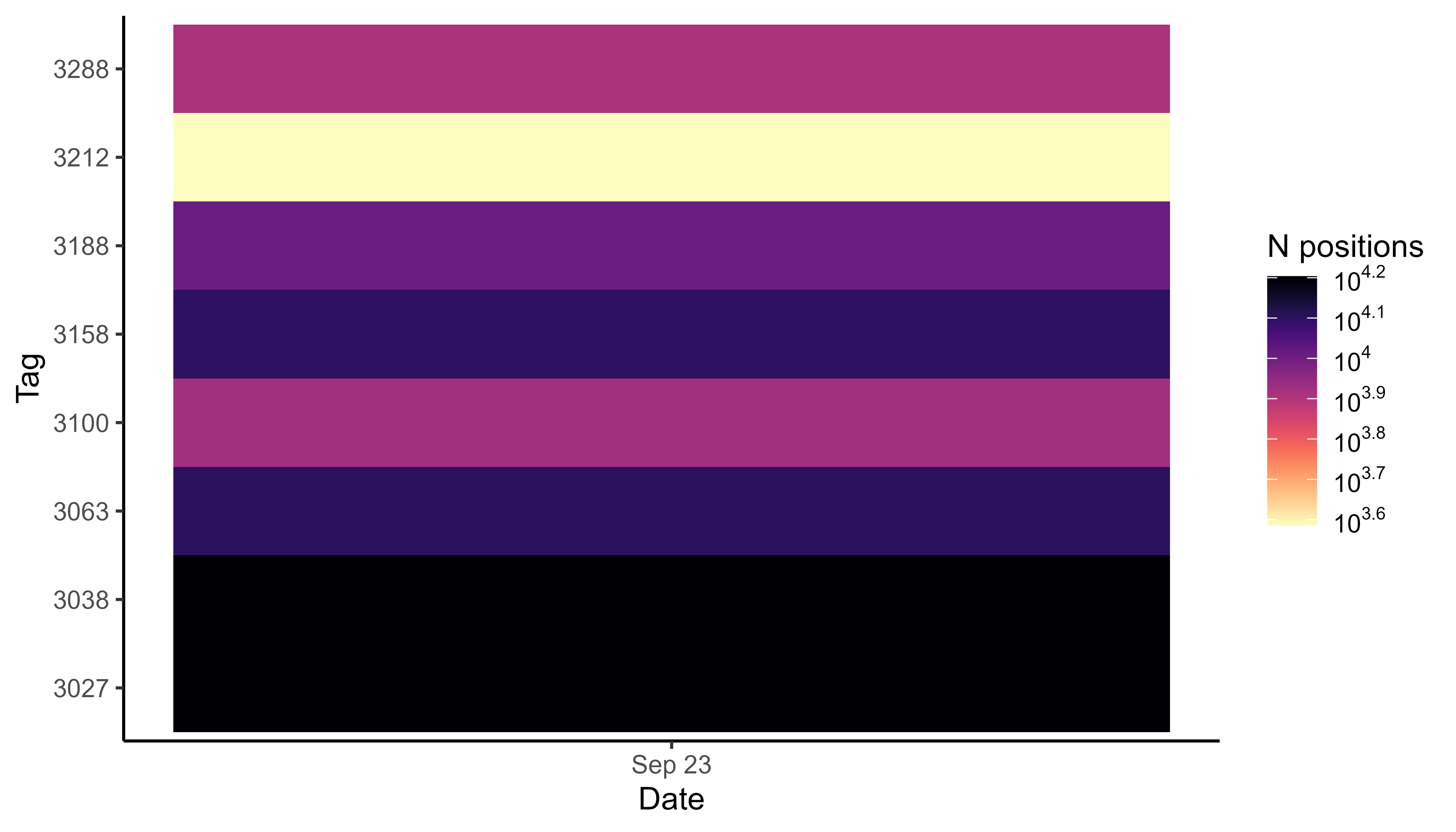

Number of positions per day by tag

Plot overview of the data

Now we want to see the data on a map. With large datasets it is convenient to plot heatmaps, as plotting for example 40 million points would result in a lot of over plotting and makes the plotting slow. If the dataset is small, one can obviously also plot the data by tag number or in other ways (see vignette plotting data).

# Make a basemap with the extent of the data
bm <- atl_create_bm(data, buffer = 1000)

# Round data to 200 m grid cells
data_heatmap <- copy(data)
data_heatmap <- data_heatmap[, c("x_round", "y_round") := list(
  plyr::round_any(x, 200),
  plyr::round_any(y, 200)
)]
data_heatmap <- data_heatmap[, .N, by = c("x_round", "y_round")]

# Plot heatmap
bm +
  geom_tile(
    data = data_heatmap, aes(x_round, y_round, fill = N),
    linewidth = 0.1, show.legend = TRUE
  ) +
  scale_fill_viridis(
    option = "A", discrete = FALSE, trans = "log10", name = "N positions",
    breaks = trans_breaks("log10", function(x) 10^x),
    labels = trans_format("log10", math_format(10^.x)),
    direction = -1
  )

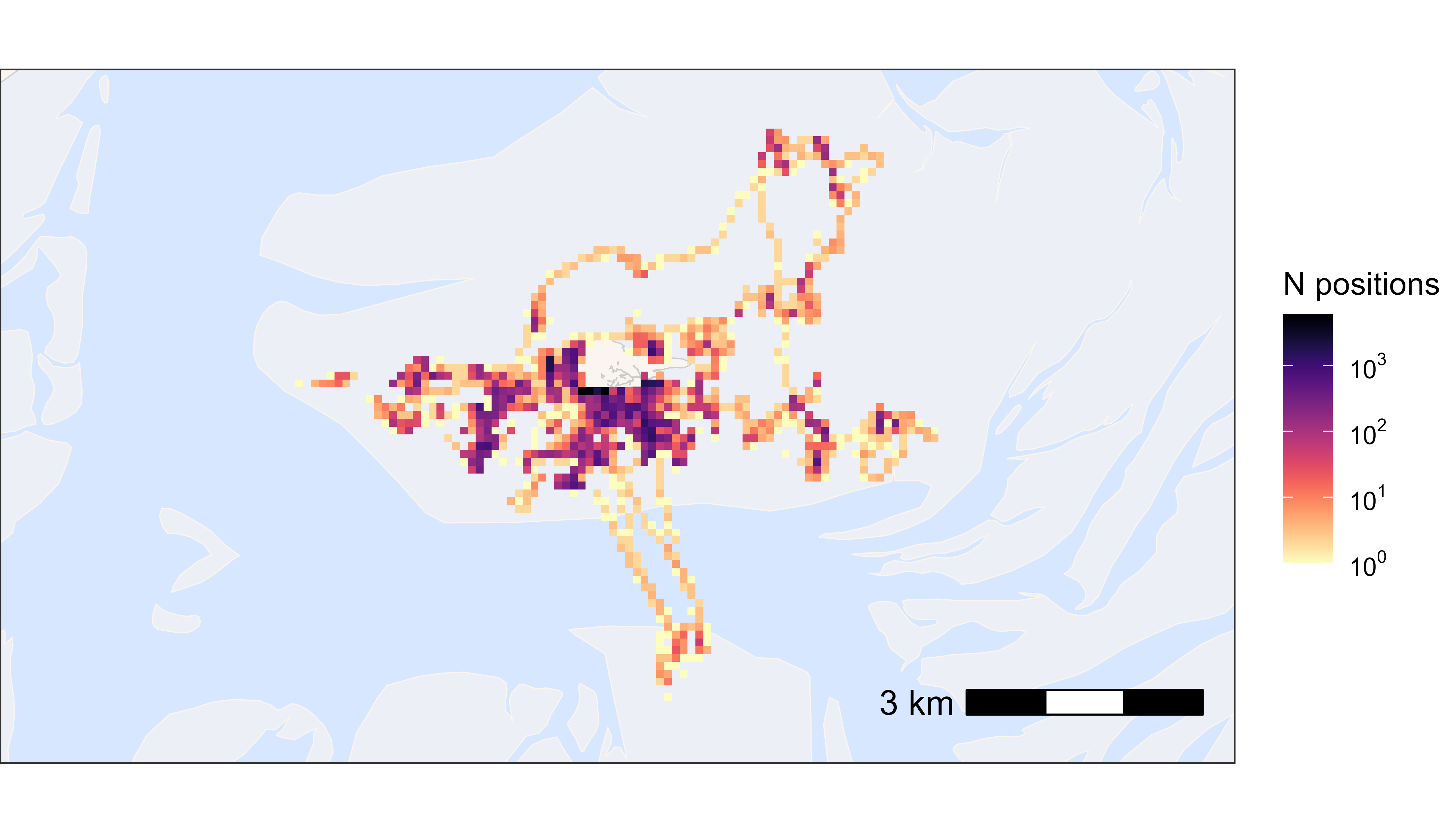
Heatmap of all positions

Johannes Krietsch