Add tidal and bathymetry data

This article shows how to add tidal and bathymetry data to WATLAS data, subset data within tidal cycle, and visualise the tracking data on the bathymetry.

Load packages and movement data

library(tools4watlas)
library(terra)
library(ggplot2)

# path to csv with aggregated data
data_path <- system.file(
  "extdata", "watlas_data_smoothed.csv",
  package = "tools4watlas"
)

# load data
data <- fread(data_path, yaml = TRUE)

Add tidal data

Tide data are from West-Terschelling and prepared by Allert. They are located in the “WATLAS” SharePoint folder: Documents/data/. Either specify the path to your local copy of this folder or add the path for your user in the atl_file_path() function.

Here we show how to add tide data (tideID - a unique tide identifier, tidaltime and time2lowtide - time from high tide and time to low tide in minutes, waterlevel - as measured from the tide gauge station with offset) in cm NAP.

# file path to WATLAS teams data folder
fp <- atl_file_path("watlas_teams")

# sub path to tide data
tidal_pattern_fp <- paste0(
  fp, "waterdata/allYears-tidalPattern-west_terschelling-UTC.csv"
)
measured_water_height_fp <- paste0(
  fp, "waterdata/allYears-gemeten_waterhoogte-west_terschelling-clean-UTC.csv"
)

# load tide data
tidal_pattern <- fread(tidal_pattern_fp)
measured_water_height <- fread(measured_water_height_fp)

# add tide data to movement data
# The offset of 30 minutes is set to match Griend.
data <- atl_add_tidal_data(
  data = data,
  tide_data = tidal_pattern,
  tide_data_highres = measured_water_height,
  waterdata_resolution = "10 min",
  waterdata_interpolation = "1 min",
  offset = 30
)

# show first 5 rows (subset of columns to show additional ones)
head(data[, .(tag, datetime, tideID, tidaltime, time2lowtide, waterlevel)]) |>
  knitr::kable(digits = 2)

tag	datetime	tideID	tidaltime	time2lowtide	waterlevel
3027	2023-09-23 03:13:25	2023513	133.42	-246.58	49.9
3027	2023-09-23 03:13:28	2023513	133.47	-246.53	49.9
3027	2023-09-23 03:19:49	2023513	139.82	-240.18	45.0
3027	2023-09-23 03:19:52	2023513	139.87	-240.13	45.0
3027	2023-09-23 03:19:55	2023513	139.92	-240.08	45.0
3027	2023-09-23 03:19:58	2023513	139.97	-240.03	45.0

Add bathymetry data

Bathymetry data can be downloaded from Rijkswaterstaat but can also be found in the “Birds, fish ’n chips” SharePoint folder: Documents/data/GIS/rasters/. To run the below script, set the file path (fp) to the local copy of the folder on your computer.

Here, we show how to extract bathymetry data (cm NAP) for each WATLAS position.

# file path to Birds, fish 'n chips GIS/rasters folder
fp <- atl_file_path("rasters")

# load bathymetry data
bat <- rast(paste0(fp, "bathymetry/2024/bodemhoogte_20mtr_UTM31_int.tif"))

# add bathymetry data
data <- atl_add_raster_data(
  data, raster_data = bat, new_name = "bathymetry", change_unit = 100 # m to cm
)

# show first 5 rows (subset of columns to show additional ones)
head(data[, .(tag, datetime, bathymetry)]) |>
  knitr::kable(digits = 2)

tag	datetime	bathymetry
3027	2023-09-23 03:13:25	84.29
3027	2023-09-23 03:13:28	84.29
3027	2023-09-23 03:19:49	86.83
3027	2023-09-23 03:19:52	86.83
3027	2023-09-23 03:19:55	86.83
3027	2023-09-23 03:19:58	86.83

Examples

Filter data by specific times within the tide cycle

To select localizations when mudlfats are available for foraging, we can for example select a low tide period from -2.5 hours to +2.5 hours around low tide (Bijleveld et al. 2016):

# select the low tide period for a particular tide as specified by tideID
data_subset <- atl_filter_covariates(
  data = data,
  filters = c(
    "tideID %in% c(2023513, 2023514)",
    "between(time2lowtide, -2.5 * 60, 2.5 * 60)"
  )
)

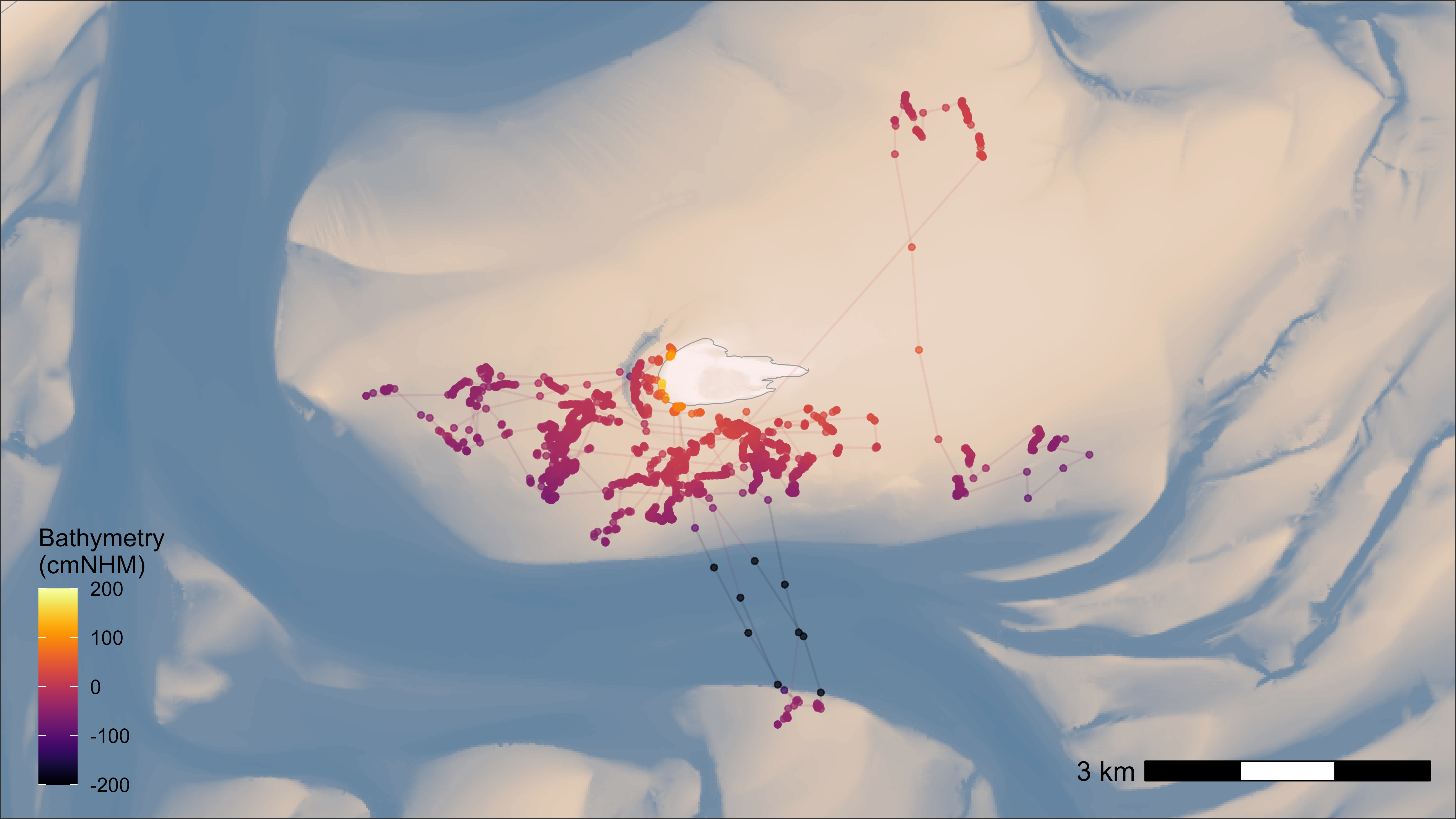
## Note: 50.18% of the dataset was filtered out, corresponding to 43596 positions.

Plot movement data on top of bathymetry layer

# additional packages
library(ggplot2)
library(viridis)
library(scales)

# file path to WATLAS teams data folder
fp <- atl_file_path("rasters")

# load bathymetry data
bat <- rast(paste0(fp, "bathymetry/2024/bodemhoogte_20mtr_UTM31_int.tif"))

# create base map with bathymetry data
bm <- atl_create_bm(
  data_subset,
  buffer = 1000, raster_data = bat, option = "bathymetry"
)

# plot data
bm +
  geom_path(
    data = data_subset, aes(x, y, group = tag, colour = bathymetry),
    alpha = 0.1, show.legend = FALSE
  ) +
  geom_point(
    data = data_subset, aes(x, y, color = bathymetry), size = 1,
    alpha = 0.7, show.legend = TRUE
  ) +
  guides(colour = guide_colourbar(position = "inside"), fill = "none") +
  scale_color_viridis(
    direction = 1, option = "inferno", name = "Bathymetry\n(cmNHM)",
    limits = c(-200, 200), oob = scales::squish
  ) +
  theme(
    legend.position.inside = c(0.07, 0.2),
    legend.background = element_rect(fill = NA)
  )