Animate data

This article gives a simple workflow on how to animate movement data. It works with any type of basemap and allows to adjust everything as wanted. It first shows how to animate data with a simple basemap and then how to do it with a bathymetry data basemap and the water level. The first two steps and the last are the same (load packages, prepare movement data, make animation).

Install mapmate from GitHub: remotes::install_github("leonawicz/mapmate").

Load packages

# packages
library(tools4watlas)
library(ggplot2)
library(viridis)
library(foreach)
library(doFuture)
library(ragg)
library(mapmate)

# additional to add water data
library(terra)
library(tidyterra)
library(sf)

Prepare movement data

Set the folder path where the png’s are created, load the data, create time steps with a desired interval (e.g. 10 min), delete existing files.

# file path
path <- "C:/Users/jkrietsch/temp/animation"

# load example data
data <- data_example

# create time steps
ts <- atl_time_steps(
  datetime_vector = data$datetime,
  time_interval = "10 min",
  output_path = path
)

# delete existing files (if any)
unlink(paste0(path, "/*"), recursive = TRUE)

Simple animation of movements

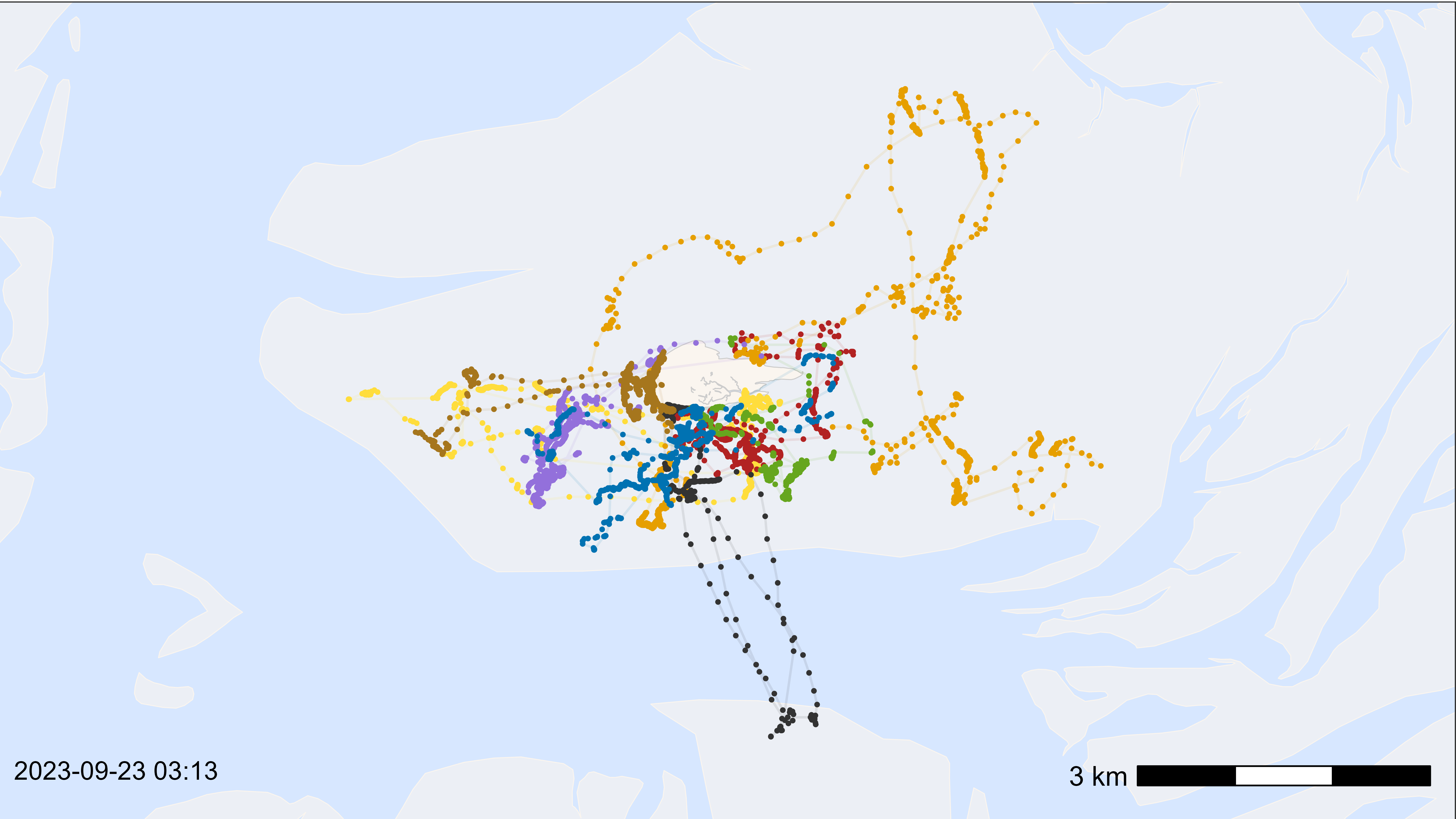
Check plot

Make a basemap as desired and plot with all data to check the outcome, scalebar and time stamp. Adjust everything as desired (check with saving png in the defined size).

# create basemap
bm <- atl_create_bm(data, buffer = 800)

# plot points and tracks to check
bm +
  geom_path(
    data = data, aes(x, y, colour = tag),
    linewidth = 0.5, alpha = 0.1, show.legend = FALSE
  ) +
  geom_point(
    data = data, aes(x, y, colour = tag),
    size = 0.5, alpha = 1, show.legend = FALSE
  ) +
  # add time stamp
  annotate(
    "text",
    x = -Inf, y = -Inf, hjust = -0.1, vjust = -2.4,
    label = paste0(format(data[1]$datetime, "%Y-%m-%d %H:%M")), size = 4
  )

Check the basemap

Loop to create png’s for each step

Create a png for each step (check steps - that is how many png’s are created). Run first with an example step to check (e.g. step <- 50) outcome for one png. Depending on the number of png’s, run first on a subset to check if everything is as desired, once everything is fine, run for all steps. A desired color scale can be simply added to p.

In the subset step, the maximal tail length can be chosen (here, 6 h). Then we use atl_alpha_along() to create an fading alpha and atl_size_along() to make a comet shape - adjust parameters as desired (see function description for more details). Afterwards we add this path to the basemap and add the time stamp.

# register cores and backend for parallel processing
registerDoFuture()
plan(multisession)

# steps
steps <- seq_len(nrow(ts))

# loop to create pngs for each time step
foreach(i = steps) %dofuture% {

  # define time step
  time_step <- ts[i]$datetime # current date

  # subset data
  ds <- data[datetime %between% c(time_step - 3600 * 6, time_step)]

  # create alpha and size
  if (nrow(ds) > 0) {
    ds[, a := atl_alpha_along(
      datetime,
      head = 30, skew = -2
    ), by = tag]
  }
  if (nrow(ds) > 0) {
    ds[, s := atl_size_along(
      datetime,
      head = 70, to = c(0.3, 2)
    ), by = tag]
  }

  # add tracks to basemap
  p <- bm +
    geom_path(
      data = ds, aes(x, y, color = tag), alpha = ds$a, linewidth = ds$s,
      lineend = "round", show.legend = FALSE
    ) +

    # add time stamp
    annotate(
      "text",
      x = -Inf, y = -Inf, hjust = -0.1, vjust = -2.4,
      label = paste0(format(time_step, "%Y-%m-%d %H:%M")), size = 4
    )

  # save png
  agg_png(
    filename = ts[i, path],
    width = 3840, height = 2160, units = "px", res = 300
  )
  print(p)
  dev.off()

}

# close parallel workers
plan(sequential)

Animation of movements with water level

Add tide and bathymetry data

We add water level data to ts to know the waterlevel at each step and crop the bathymetry data to the extend of the map (use same buffer as for basemap).

# file path to WATLAS teams data folder
fp <- atl_file_path("watlas_teams")

# sub path to tide data
tidal_pattern_fp <- paste0(
  fp, "waterdata/allYears-tidalPattern-west_terschelling-UTC.csv"
)
measured_water_height_fp <- paste0(
  fp, "waterdata/allYears-gemeten_waterhoogte-west_terschelling-clean-UTC.csv"
)

# load tide data
tidal_pattern <- fread(tidal_pattern_fp)
measured_water_height <- fread(measured_water_height_fp)

# add unix time
ts[, time := as.numeric(datetime)]

# add tide data to movement data
ts <- atl_add_tidal_data(
  data = ts,
  tide_data = tidal_pattern,
  tide_data_highres = measured_water_height,
  waterdata_resolution = "10 min",
  waterdata_interpolation = "1 min",
  offset = 30
)

# file path to Birds, fish 'n chips GIS/rasters folder
fp <- atl_file_path("rasters")

# load bathymetry data
bat <- rast(paste0(fp, "bathymetry/2024/bodemhoogte_20mtr_UTM31_int.tif"))

# bbox (should be buffer used for basemap)
bbox <- atl_bbox(data, buffer = 800)

# crop the raster using the bounding box
bat_c <- crop(bat, bbox)

# wrap to use in parallel loop
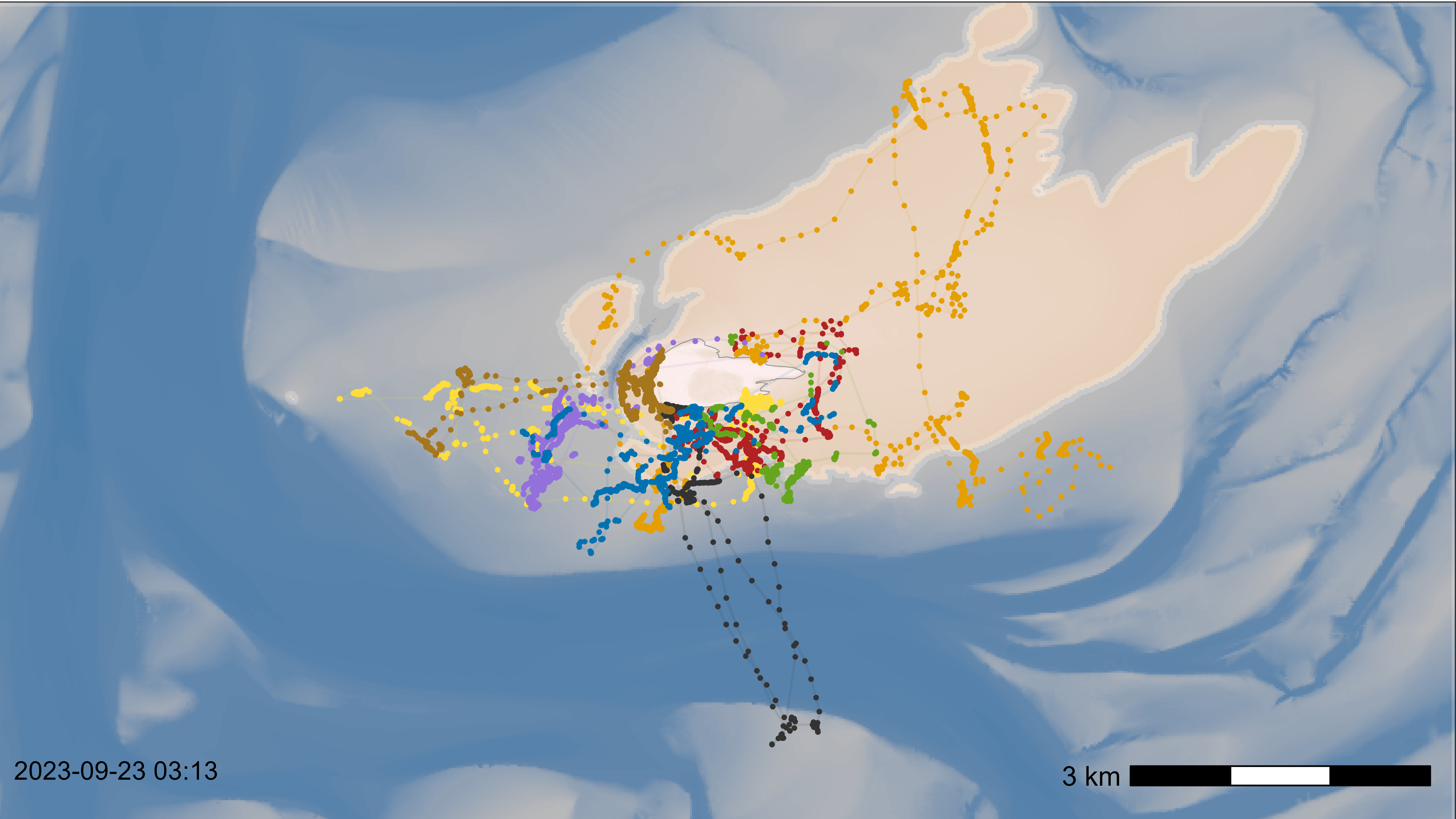
bat_w <- wrap(bat_c)

Check plot

Make a basemap as desired and plot with all data to check the outcome, scalebar and time stamp. Adjust everything as desired (check with saving png in the defined size).

# create basemap
bm <- atl_create_bm(
  data,
  buffer = 800, raster_data = bat_c, option = "bathymetry", scalebar = FALSE
)

# extract example water level
threshold <- 0 / 100 # water level at the time (/100 to scale to m)
bat_m <- bat_c < threshold # mask below threshold (TRUE = 1)
bat_m[bat_m == 0] <- NA # remove land
waterline <- as.polygons(bat_m, values = TRUE, dissolve = TRUE) |>
  st_as_sf() # extract polygon with water level

# check plot with all data
bm +
  # add water level
  geom_sf(
    data = waterline, fill = "dodgerblue3", alpha = 0.2,
    color = scales::alpha("white", 0.2), linewidth = 2
  ) +
  # add points and tracks
  geom_path(
    data = data, aes(x, y, colour = tag),
    linewidth = 0.5, alpha = 0.1, show.legend = FALSE
  ) +
  geom_point(
    data = data, aes(x, y, colour = tag),
    size = 0.5, alpha = 1, show.legend = FALSE
  ) +
  # add time stamp
  annotate(
    "text",
    x = -Inf, y = -Inf, hjust = -0.1, vjust = -2.4,
    label = paste0(format(data[1]$datetime, "%Y-%m-%d %H:%M")), size = 4
  ) +
  # add scale bar
  ggspatial::annotation_scale(
    aes(location = "br"),
    text_cex = 1, height = unit(0.3, "cm"),
    pad_x = unit(0.4, "cm"), pad_y = unit(0.6, "cm")
  ) +
  # set extend again (overwritten by geom_sf)
  coord_sf(
    xlim = c(bbox["xmin"], bbox["xmax"]),
    ylim = c(bbox["ymin"], bbox["ymax"]), expand = FALSE
  )

Check the basemap with bathymetry data

Loop to create png’s for each step

Same as above just with added water level polygon and scale bar (needs to be added above water).

# register cores and backend for parallel processing
registerDoFuture()
plan(multisession)

# steps
steps <- seq_len(nrow(ts))

# loop to create pngs for each time step
foreach(i = steps) %dofuture% {

  # define time step
  time_step <- ts[i]$datetime # current date

  # subset data
  ds <- data[datetime %between% c(time_step - 3600 * 6, time_step)]

  # create alpha and size
  if (nrow(ds) > 0) {
    ds[, a := atl_alpha_along(
      datetime,
      head = 30, skew = -2
    ), by = tag]
  }
  if (nrow(ds) > 0) {
    ds[, s := atl_size_along(
      datetime,
      head = 70, to = c(0.3, 2)
    ), by = tag]
  }

  # extract water level
  bat_c <- unwrap(bat_w)
  threshold <- ts[i]$waterlevel / 100 # water level at the time (scale to m)
  bat_m <- bat_c < threshold # mask below threshold (TRUE = 1)
  bat_m[bat_m == 0] <- NA # remove land
  waterline <- as.polygons(bat_m, values = TRUE, dissolve = TRUE) |>
    st_as_sf() # extract polygon with water level

  # add everything to the basemap
  p <- bm +
    # add water level
    geom_sf(
      data = waterline, fill = "dodgerblue3", alpha = 0.2,
      color = scales::alpha("white", 0.2), linewidth = 2
    ) +
    # add track
    geom_path(
      data = ds, aes(x, y, color = tag), alpha = ds$a, linewidth = ds$s,
      lineend = "round", show.legend = FALSE
    ) +
    # add time stamp
    annotate(
      "text",
      x = -Inf, y = -Inf, hjust = -0.1, vjust = -2.4,
      label = paste0(format(time_step, "%Y-%m-%d %H:%M")), size = 4
    ) +
    # add scale bar
    ggspatial::annotation_scale(
      aes(location = "br"),
      text_cex = 1, height = unit(0.3, "cm"),
      pad_x = unit(0.4, "cm"), pad_y = unit(0.6, "cm")
    ) +
    # set extend again (overwritten by geom_sf)
    coord_sf(
      xlim = c(bbox["xmin"], bbox["xmax"]),
      ylim = c(bbox["ymin"], bbox["ymax"]), expand = FALSE
    )

  # save png
  agg_png(
    filename = ts[i, path],
    width = 3840, height = 2160, units = "px", res = 300
  )
  print(p)
  dev.off()

}

# close parallel workers
plan(sequential)

Make a animation using `ffmpeg` via `mapmate`

Adjust the frame rate (rate) as desired (depending on the time step interval). File is created in the same path, but this can also be changed as desired.

# make animation
ffmpeg(
  dir = path, output_dir = path, pattern = atl_ffmpeg_pattern(ts[1]$path),
  output = "Animation.mp4", rate = 8, details = TRUE, overwrite = TRUE
)

Johannes Krietsch

Load packages

Prepare movement data

Simple animation of movements

Check plot

Loop to create png’s for each step

Animation of movements with water level

Add tide and bathymetry data

Check plot

Loop to create png’s for each step

Make a animation using ffmpeg via mapmate

Make a animation using `ffmpeg` via `mapmate`