Basemap data

Johannes Krietsch

This script shows how to create the basemap data of tools4watlas, which are a land polygon of the Dutch Wadden Sea, the mudflats of North Holland and Friesland and waterbodies on Griend. These data were choosen provide a simple map with relevant data allowing fast plotting. Customized basemap data could be created in a similar way and could additional contain buildings, roads, lakes, rivers etc. All data can be found in the “Birds, fish ’n chips” SharePoint folder: Documents/data/GIS/shapefiles/. To run the script set the file path (wd) to the local copy of the folder on your computer.

The OpenStreetMap land polygon can also be downloaded from osmdata and the regional data of the Netherlands (here used are North Holland and Friesland) can be downloaded from Geofabrik.

Load packages and specify path to local data

# Packages
library(data.table)
library(tools4watlas)
library(sf)
library(ggplot2)
library(rnaturalearth)
library(rnaturalearthdata)

# path to folder with local shapefiles
wd <- "C:/Users/jkrietsch/OneDrive - NIOZ/Documents/map_data/"

Define a bounding box of the Dutch Wadden Sea

First define a bounding box which is used to crop the land polygon data.

# get data from the Netherlands
netherlands <- ne_countries(
  country = "netherlands", scale = "large", returnclass = "sf"
) |>
  st_transform(crs = st_crs(32631))

# point of Griend (and a bit east)
griend <- st_sfc(st_point(c(5.2525 + 0.3, 53.2523)), crs = st_crs(4326)) |>
  st_transform(crs = st_crs(32631))

# bounding box around Griend
bbox <- atl_bbox(griend, asp = "16:9", buffer = 45000)
bbox_sf <- bbox |> st_as_sfc()

# plot
ggplot() +
  geom_sf(data = netherlands) +
  geom_sf(data = bbox_sf, color = "firebrick3", fill = NA) +
  coord_sf(
    xlim = c(bbox["xmin"], bbox["xmax"]),
    ylim = c(bbox["ymin"], bbox["ymax"])
  )

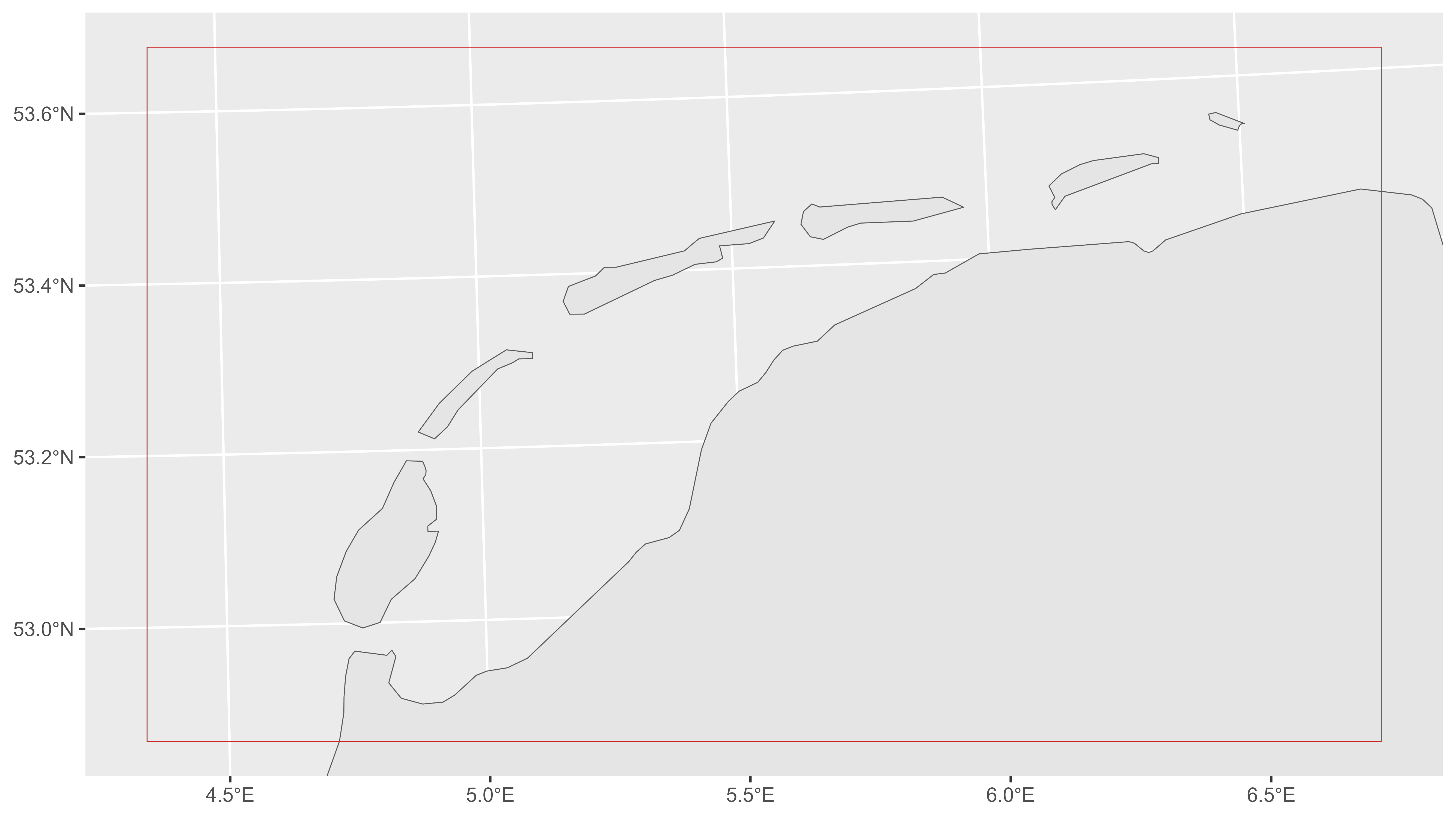
Bounding box around the Dutch Wadden Sea

Extract the land polygon data from this bounding box

# load osm land polygon
land_ <- st_read(quiet = TRUE, paste0(
  wd, "open_street_map/land-polygons-complete-4326/land_polygons.shp"
)) |>
  st_transform(crs = st_crs(32631))

# crop data
land <- st_intersection(land_, bbox_sf)

# extract only geometry
land <- land["geometry"]

# union to compress
land <- st_union(land)

# plot
ggplot() +
  geom_sf(data = land) +
  geom_sf(data = bbox_sf, color = "firebrick", fill = NA) +
  coord_sf(
    xlim = c(bbox["xmin"], bbox["xmax"]),
    ylim = c(bbox["ymin"], bbox["ymax"])
  )

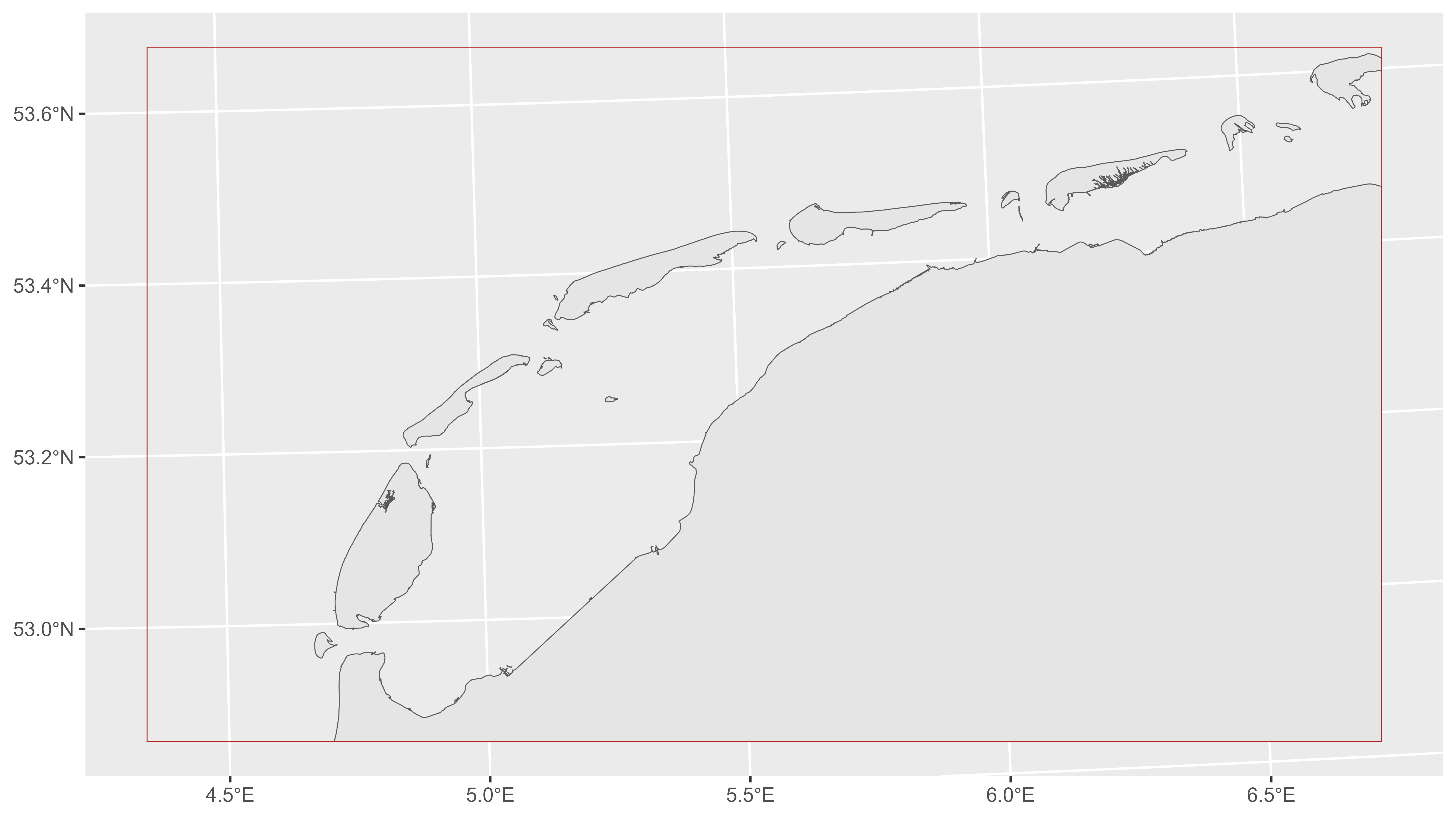
Cropped land polygon around the Dutch Wadden Sea

Save data

Includes data in the package, if tools4watlas is opened as project.

# save data
save(land, file = "../../data/land.rda", compress = "xz")

Define a polygon of the Dutch Wadden Sea

To simplify the basemap we only want the mudflats from within the Wadden Sea, otherwise fclass also includes other wetlands.

# load polygon of Wadden sea
wadden_sea <- st_read(quiet = TRUE, paste0(
  wd, "wadden_area_legally/pkb_gebied_derde_nota_waddenzee.shp"
)) |>
  st_transform(crs = st_crs(32631))

# crop with bbox
wadden_sea <- st_intersection(wadden_sea, bbox_sf)

# buffer
ws_buffer <- wadden_sea |> st_buffer(1000)
ws_buffer <- ws_buffer[, c("geometry")]

# check data
ggplot() +
  geom_sf(data = land) +
  geom_sf(data = ws_buffer, color = "firebrick", fill = NA)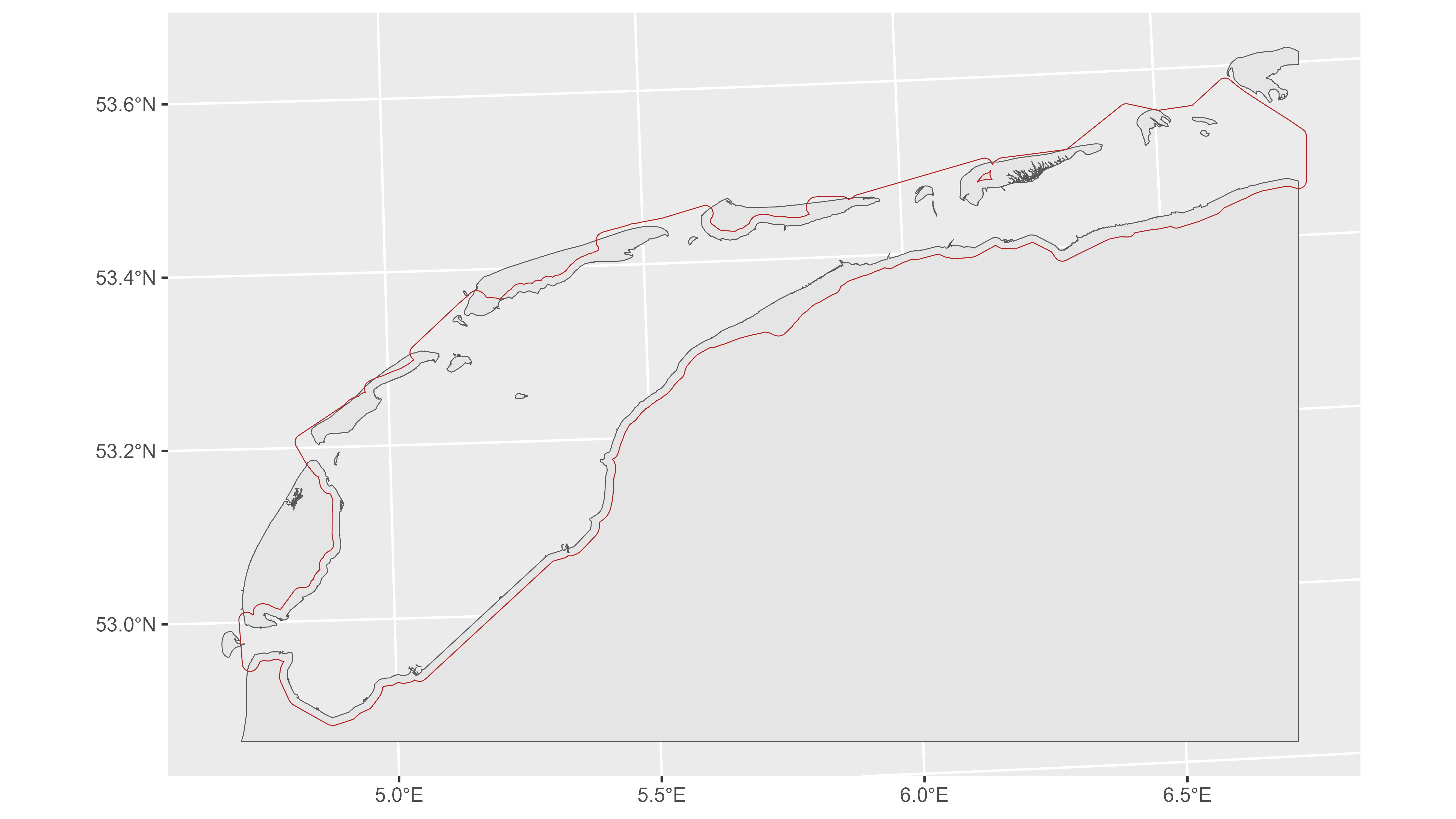

Polygon of the Dutch Wadden Sea

Extract mudflats and lakes from within the Wadden Sea

We only take the lakes from Griend to not blow up the data.

# Friesland
lakes_fr <- st_read(quiet = TRUE, paste0(
  wd, "open_street_map/friesland-latest-free.shp/gis_osm_water_a_free_1.shp"
))

# North Holland
lakes_nh <- st_read(quiet = TRUE, paste0(
  wd, "open_street_map/noord-holland-latest-free.shp/gis_osm_water_a_free_1.shp"
))

# merge both and change projection
lakes_ <- rbind(lakes_fr, lakes_nh) |>
  unique(by = "osm_id") |>
  st_transform(crs = st_crs(32631))

# crop data
lakes <- st_intersection(lakes_, ws_buffer)

# subset mudflats
mudflats <- lakes[lakes$fclass == "wetland", ]

# union to compress
mudflats <- st_union(mudflats)

# subset lakes
lakes <- lakes[lakes$fclass == "water", ]

# crop to include just Griend
griend <- st_sfc(st_point(c(5.2525, 53.2523)), crs = st_crs(4326)) |>
  st_transform(crs = st_crs(32631))
bbox_sf <- atl_bbox(griend, asp = "16:9", buffer = 3000) |> st_as_sfc()
lakes <- st_intersection(lakes, bbox_sf)

# union to compress
lakes <- st_union(lakes)

# plot
ggplot() +
  geom_sf(
    data = mudflats, fill = "#faf5ef", alpha = 0.6, colour = "#faf5ef"
  ) +
  geom_sf(data = land, fill = "#faf5ef", colour = "grey80") +
  geom_sf(
    data = lakes, fill = "#D7E7FF", colour = "grey80"
  ) +
  coord_sf(
    xlim = c(bbox["xmin"], bbox["xmax"]),
    ylim = c(bbox["ymin"], bbox["ymax"]),
    expand = FALSE
  ) +
  theme(
    panel.grid.major = element_line(colour = "transparent"),
    panel.grid.minor = element_line(colour = "transparent"),
    panel.background = element_rect(fill = "#D7E7FF"),
    plot.background = element_rect(fill = "transparent", colour = NA),
    panel.border = element_rect(fill = NA, colour = "grey20")
  )

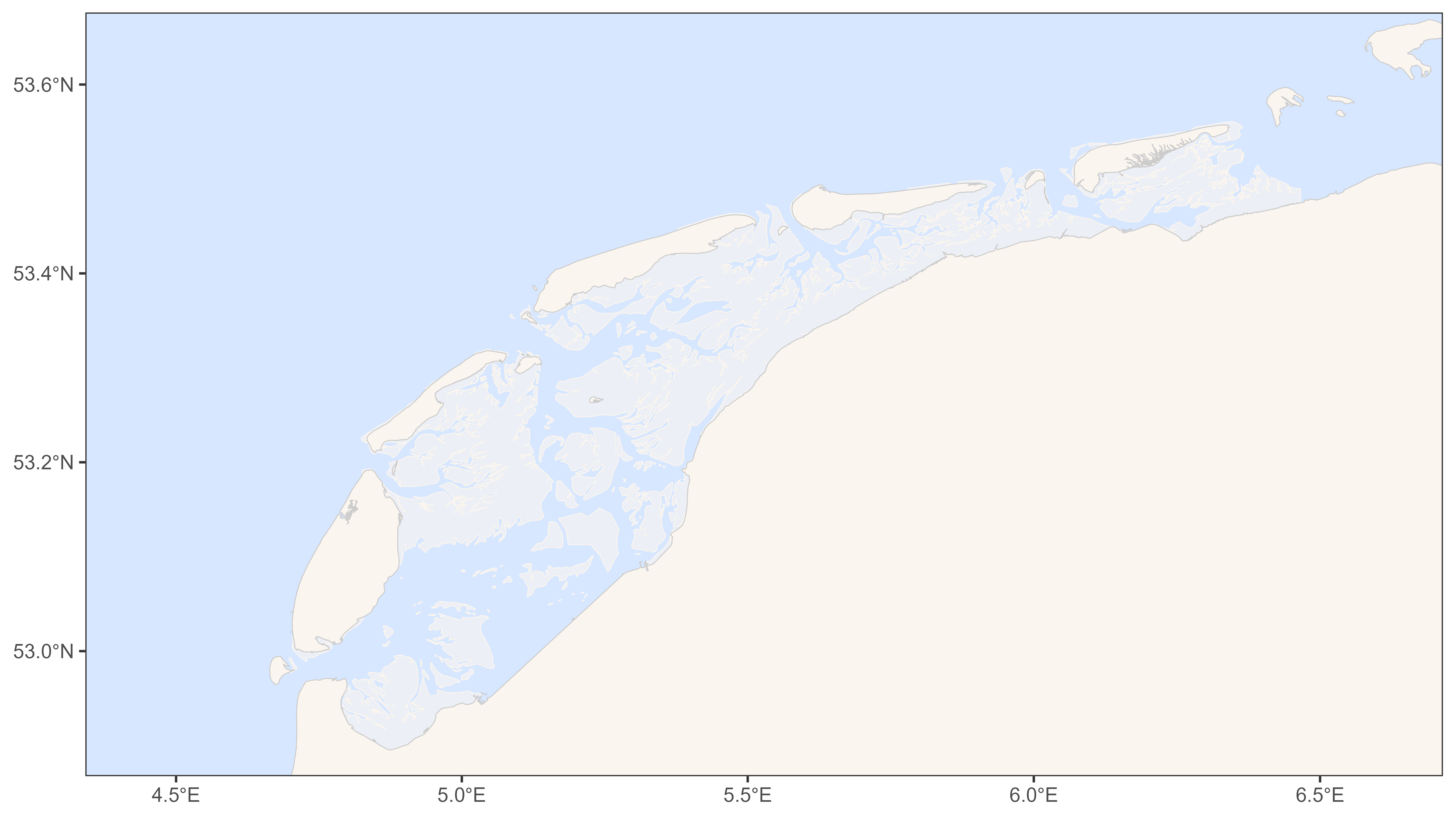
Final basemap data of the Dutch Wadden Sea

Save data

Includes data in the package, if tools4watlas is opened as project.

# save data
save(mudflats, file = "../../data/muddflats.rda", compress = "xz")
save(lakes, file = "../../data/lakes.rda", compress = "xz")