Interpolate data • tools4watlas

This article shows how to interpolate WATLAS data and how to create relative distributions. Interpolation should be used mindful and with consideration of the data and research question. Some analysis need regular spaced data and given temporal and spatial restrictions, interpolation can be a useful tool to fill in gaps in the data. For example, if the data are collected at irregular intervals, interpolation can be used to create a regular time series of positions. For example, within residence patches, when birds are on the ground, especially when roosting, it is likely that the bird is not moving much and in this case an interpolation can be useful to create data that better describe the space use in association with time. One could also simply use the median residency patch position and the time spent in the patch, but this would not allow to capture the space use within the residence patch.

Load packages and required data

# packages
library(tools4watlas)
library(ggplot2)
library(viridis)
library(foreach)
library(doFuture)

# load example data
data <- data_example

Prepare data by calculating residence patches and thinning

We first need to calculate residence patches as described in the article “Add residence patches” and thin the data to a regular interval as described in the article “Smooth and thin data”.

# subset relevant columns
data <- data[, .(species, posID, tag, time, datetime, x, y, tideID)]

# extract the unique tag IDs
id <- unique(data$tag)

# register cores and backend for parallel processing
registerDoFuture()
plan(multisession)

# loop through all tags to calculate residence patches
data <- foreach(i = id, .combine = "rbind") %dofuture% {
  atl_res_patch(
    data[tag == i],
    max_speed = 3, lim_spat_indep = 75, lim_time_indep = 180,
    min_fixes = 3, min_duration = 120
  )
}

# close parallel processing
plan(sequential)

# summary of residence patches
data_summary <- atl_res_patch_summary(data)

# thin the data to 1 min intervall
data <- atl_thin_data(
  data = data,
  interval = 60,
  id_columns = c("tag", "species"),
  method = "aggregate"
)

Check data

Before interpolation, it is good to have an look at the residence patch summary to understand the data and to check whether interpolation is appropriate. For example, if the maximum duration of residence patches is very long, there might be a mistake in the residence patch calculation.

# merge species to data_summary
data_summary <- merge(data_summary, unique(data[, .(tag, species)]), by = "tag")

# look at the maximal length of residence patches per species
data_summary[, .(
  max_duration = max(duration) |> atl_format_time()
), by = species]

##              species max_duration
##               <char>       <char>
## 1:          redshank    2.7 hours
## 2:          red knot    5.1 hours
## 3: bar-tailed godwit    3.4 hours
## 4:            curlew    2.4 hours
## 5:     oystercatcher    7.6 hours
## 6:         turnstone    3.4 hours
## 7:            dunlin      2 hours
## 8:        sanderling      3 hours

The oystercatcher spent 7.6 h in a residence patch, which is quite long, but possible.

Interpolate data within patch

In these case, we trust the residence patch calculation and we want to interpolate the data to 1 min intervals only within residence patches. We set the max_gap to 8 h, which is longer than the longest residence patch duration, so that all residence patches are interpolated and we set patches_only to TRUE, so that only data within residence patches are interpolated.

# interpolate data to 1 min intervals only within residence patches
data_int <- atl_interpolate_track(
  data = data,
  tag = "tag",
  x = "x",
  y = "y",
  time = "time",
  patch = "patch",
  interp_interval = 60,
  max_gap = 3600 * 8,
  max_dist = NULL,
  patches_only = TRUE
)

## Note: Interpolation added 1919 positions (28.74% increase).

# show head of the table
head(data_int) |> knitr::kable(digits = 2)

tag	time	datetime	x	y	patch	gap_next	interpolated
3027	1695438780	2023-09-23 03:13:00	650705.6	5902556	1	0	FALSE
3027	1695438840	2023-09-23 03:14:00	650708.4	5902557	1	360	TRUE
3027	1695438900	2023-09-23 03:15:00	650711.1	5902558	1	360	TRUE
3027	1695438960	2023-09-23 03:16:00	650713.9	5902559	1	360	TRUE
3027	1695439020	2023-09-23 03:17:00	650716.6	5902560	1	360	TRUE
3027	1695439080	2023-09-23 03:18:00	650719.3	5902561	1	360	TRUE

Plot the data to check interpolated points

Plot one tag as example. The points are coloured by residence patch and the interpolated points are shown in black.

# subset one tag
data_subset <- data_int[tag == "3288"]

# create basemap
bm <- atl_create_bm(data_subset, buffer = 800)

# plot points and tracks with standard ggplot colours
bm +
  geom_path(
    data = data_subset, aes(x, y),
    linewidth = 0.5, alpha = 0.1, show.legend = FALSE
  ) +
  geom_point(
    data = data_subset, aes(x, y, colour = patch),
    size = 1, alpha = 1, show.legend = FALSE
  ) +
  geom_point(
    data = data_subset[interpolated == TRUE], aes(x, y), color = "black",
    size = 0.5, alpha = 1, show.legend = FALSE
  )

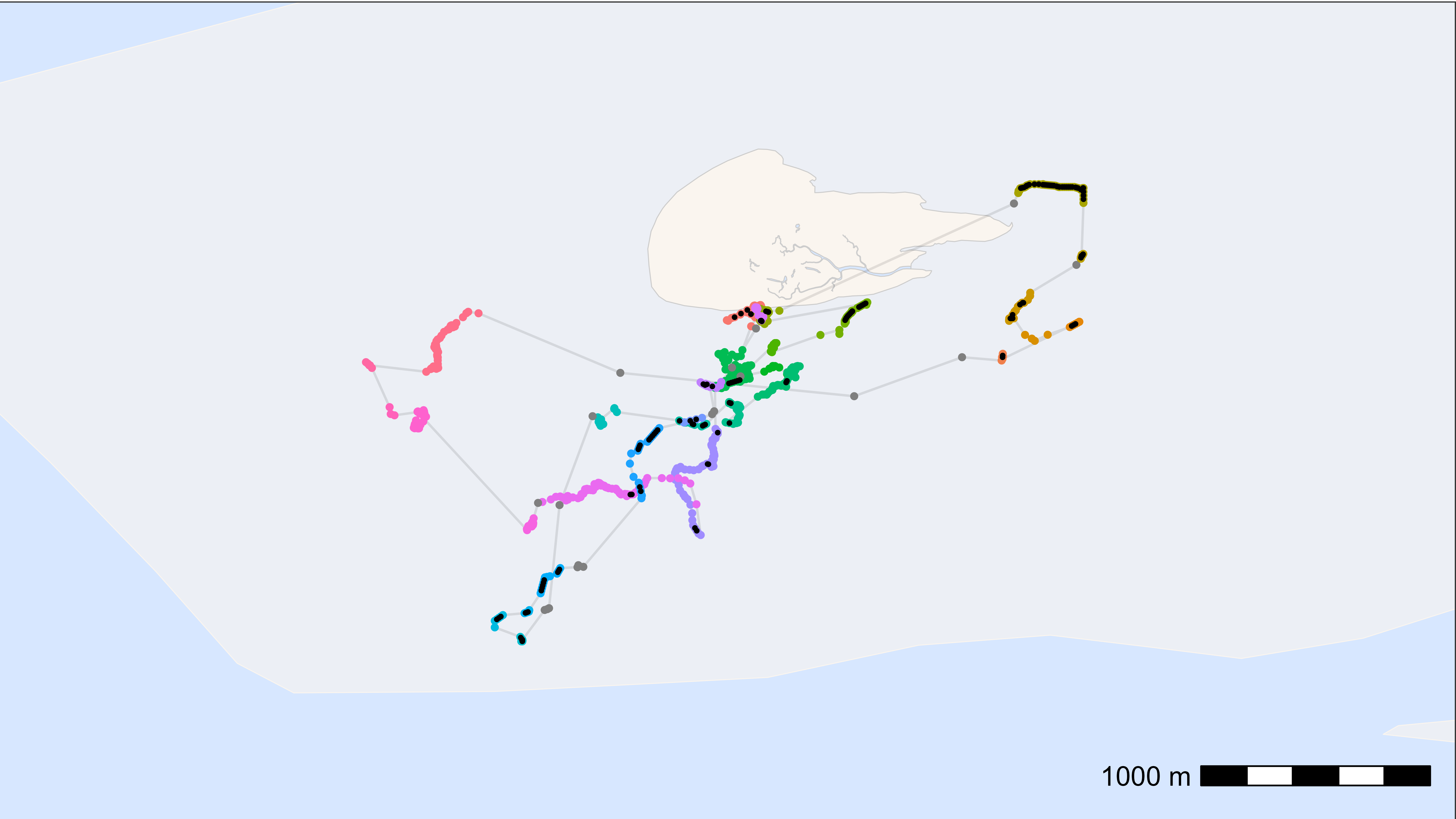
Looks good!