Add residence patches

In this vignette, we provide a general workflow to group WATLAS position data into so-called ‘residence patches’.

Background

The atl_res_patch() function is designed to segment and aggregate WATLAS movement data into residence patches. The main parameter is speed max_speed. With perfect data that would be the only parameter necessary to adjust, because the speed flying, walking or standing do not overlap. Because WATLAS data have localization error (which is comparable to GPS, see Beardsworth et al. 2022) and gaps when birds are not detected by receivers, we need to have additional variables for classifying these data into robust residence patches.

The logic of the function is to first identify proto-patches (preliminary residence patches). Subsequent positions are assigned to the same proto-patch when they have a speed smaller than max_speed, a distance smaller than lim_spat_indep and a time gap smaller than lim_time_indep. Proto-patches with fewer than min_fixes positions and shorter than min_duration are filtered out.

For each proto-patch, the median position is calculated as well as the time between subsequent proto-patches (i.e. the time between the last position of a proto-patch and the first position of the next proto-patch). If the distance between the median positions of two subsequent proto-patches is smaller than lim_spat_indep and the time between the proto-patch is less then lim_time_indep, proto-patches are merged into residence patches.

Lastly, a unique patch ID is assigned to each residence patch ordered by time from 1 to n.

Note that position error in combination with short intervals between positions (e.g. 3 sec) can lead to speed outliers that affect the creation of proto-patches. Therefore, it is recommended to first filter (e.g. var_max < 5000) and smooth (e.g. moving_window = 5) the data.

Parameter overview

Deciding on the optimal parameters for the residence patch classification is not a trivial task. The key is to find a good balance between true and false positives. See section below on how we decided on the standard parameter settings.

• max_speed: A numeric value specifying the maximum speed (m/s) between two subsequent positions that would be considered non-transitory. 3 m/s seems to be the best compromise. Higher values often result in the merging of patches with clear flights in between and with lower values clear foraging behaviour is sometimes not picked up.
• lim_spat_indep: A numeric value specifying the maximum distance (m) between subsequent residence patches for them to be considered independent. In combination with lim_time_indep, this parameter avoids making a new proto-patch from gaps in the data when the bird was actually still at the same location. 75 m seems to be the best compromise.
• lim_time_indep: A numeric value specifying the time difference (min) between two subsequent residence patches for them to be considered independent. In combination with lim_spat_indep, this parameter can prevent the creation new proto-patches when there are large gaps in the data. For example, at the roost site a bird might not move for a long time at a location with poor coverage by receivers. If the bird then moves away and sends data from the same position, we can assume that all missed positions were also at this place. 180 min (3 hours) works fine for foraging, but it could be increased with position data that has large gaps. For example, when the analysis is focused on roosting behaviour, this could even be increased to e.g. 12 hours, to deal with large gaps in the data that can occur with roosting birds not moving and being at the same place with bad signal strength.
• min_fixes: The minimum number of positions for proto-patches. To make sure that residence patches have at least a few positions. 2 positions works best in picking up proto-patches. If the patch is below min_duration it will anyway be filtered out.
• min_duration: The minimum duration (s) for classifying residence patches. With a high-sampling interval (e.g. 3 s), short residence patches can be created, which are not biological relevant. A value of 60 sec (1 minute) helps to pick-up proto-patches. Biological relevance depends on the focus of the analysis and residence patches with a shorter duration can still be filtered out afterwards.

Example workflow

Load packages and required data

Note that access to the tidal data on WATLAS-Teams is required for running this code.

# packages
library(tools4watlas)
library(ggplot2)
library(viridis)
library(patchwork)
library(foreach)
library(doFuture)

# load example data
data <- data_example

# file path to WATLAS teams data folder
fp <- atl_file_path("watlas_teams")

# sub path to tide data
tidal_pattern_fp <- paste0(
  fp, "waterdata/allYears-tidalPattern-west_terschelling-UTC.csv"
)
measured_water_height_fp <- paste0(
  fp, "waterdata/allYears-gemeten_waterhoogte-west_terschelling-clean-UTC.csv"
)

# load tide data
tidal_pattern <- fread(tidal_pattern_fp)
measured_water_height <- fread(measured_water_height_fp)

Calculate residence patches by tag

To reduce the memory size for parallel computing, we will first subset the relevant columns from the data. This could be skipped for small data tables. We will then run atl_res_patch() for each tag ID in parallel. The column patch is added to the data table, which provides the assigned patch ID’s for the positions.

# subset relevant columns
data <- data[, .(species, posID, tag, time, datetime, x, y, tideID)]

# extract the unique tag IDs
id <- unique(data$tag)

# register cores and backend for parallel processing
registerDoFuture()
plan(multisession)

# loop through all tags to calculate residence patches
data <- foreach(i = id, .combine = "rbind") %dofuture% {
  atl_res_patch(
    data[tag == i],
    max_speed = 3, lim_spat_indep = 75, lim_time_indep = 180,
    min_fixes = 2, min_duration = 60
  )
}

# close parallel processing
plan(sequential)

# show head of the summary table
head(data) |> knitr::kable(digits = 2)

species	posID	tag	time	datetime	x	y	tideID	patch
redshank	2	3027	1695438805	2023-09-23 03:13:25	650705.6	5902556	2023513	1
redshank	3	3027	1695438808	2023-09-23 03:13:28	650705.6	5902556	2023513	1
redshank	4	3027	1695439189	2023-09-23 03:19:49	650721.0	5902559	2023513	1
redshank	5	3027	1695439192	2023-09-23 03:19:52	650721.1	5902559	2023513	1
redshank	6	3027	1695439195	2023-09-23 03:19:55	650723.1	5902564	2023513	1
redshank	7	3027	1695439198	2023-09-23 03:19:58	650723.1	5902564	2023513	1

Evaluate residence-patch assignment

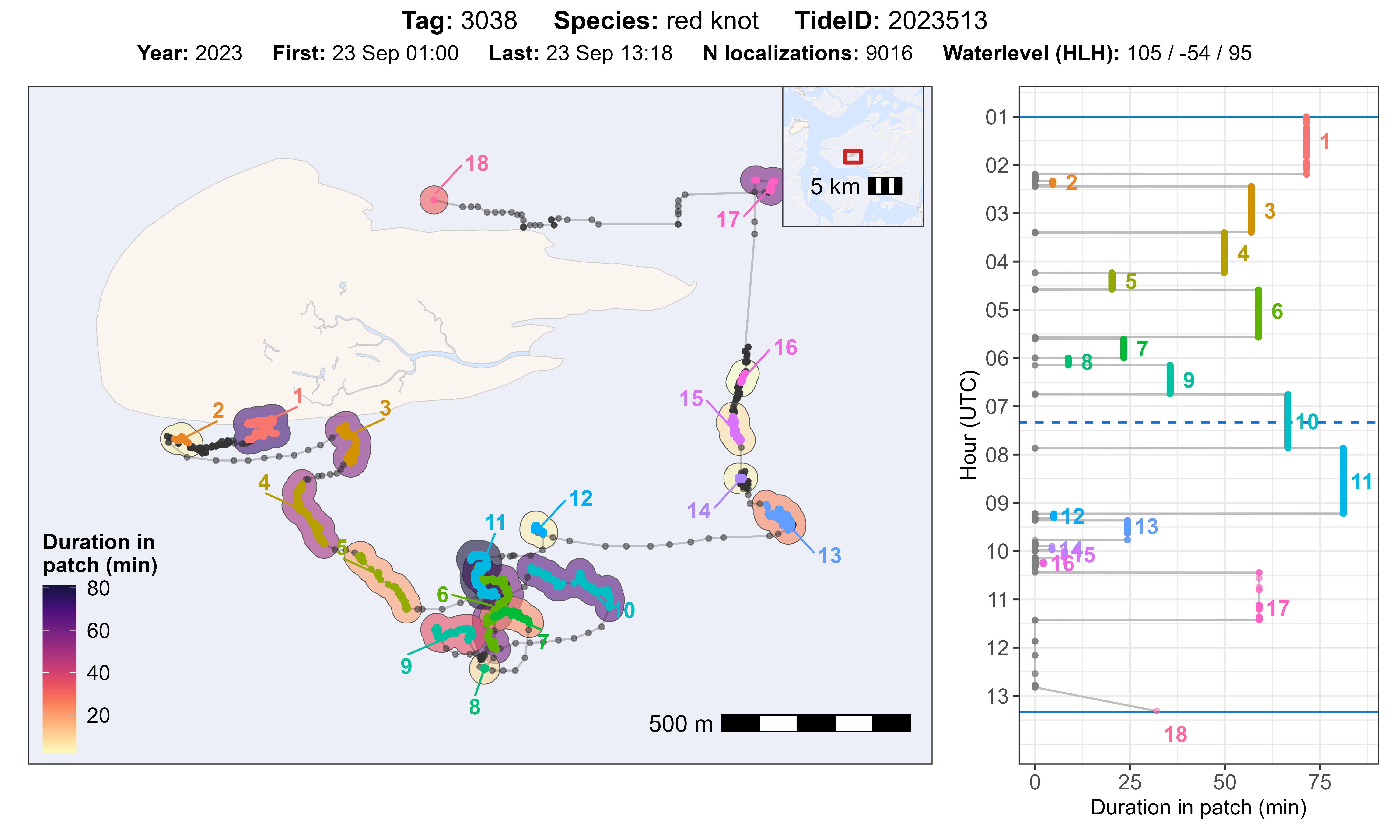
The function atl_check_res_patch() can be used to evaluate the residence patch assignment by tag and tide ID. The function plots the track with residence patches on a map and shows the duration (time in a patch in min) as coloured polygon on the map and against time in a separate panel. Time starts on the top and goes from high tide to the next high tide (solid blue lines), as well as indicating low tide (dashed blue line). The title of the plot gives basic information about the data and the water level for the corresponding tide.

Inspect one tag and tide

We can select one tag and tide to plot. Additionally, we need to specify the offset for the tidal data we use (e.g. 30 min for West-Terschelling) and a buffer (in m) around the residence patch data to create the polygon (for visualisation purposes only). For data inspection, it makes sense to set the buffer to half of lim_spat_indep (maximum distance between subsequent residence patches at which they will be considered independent), ensuring that the polygons around residence patches correspond to the spatial distance threshold used to merge residence patches.

atl_check_res_patch(
  data[tag == "3038"],
  tide_data = tidal_pattern, tide_data_highres = measured_water_height,
  tide = "2023513", offset = 30,
  buffer_res_patches = 75 / 2
)

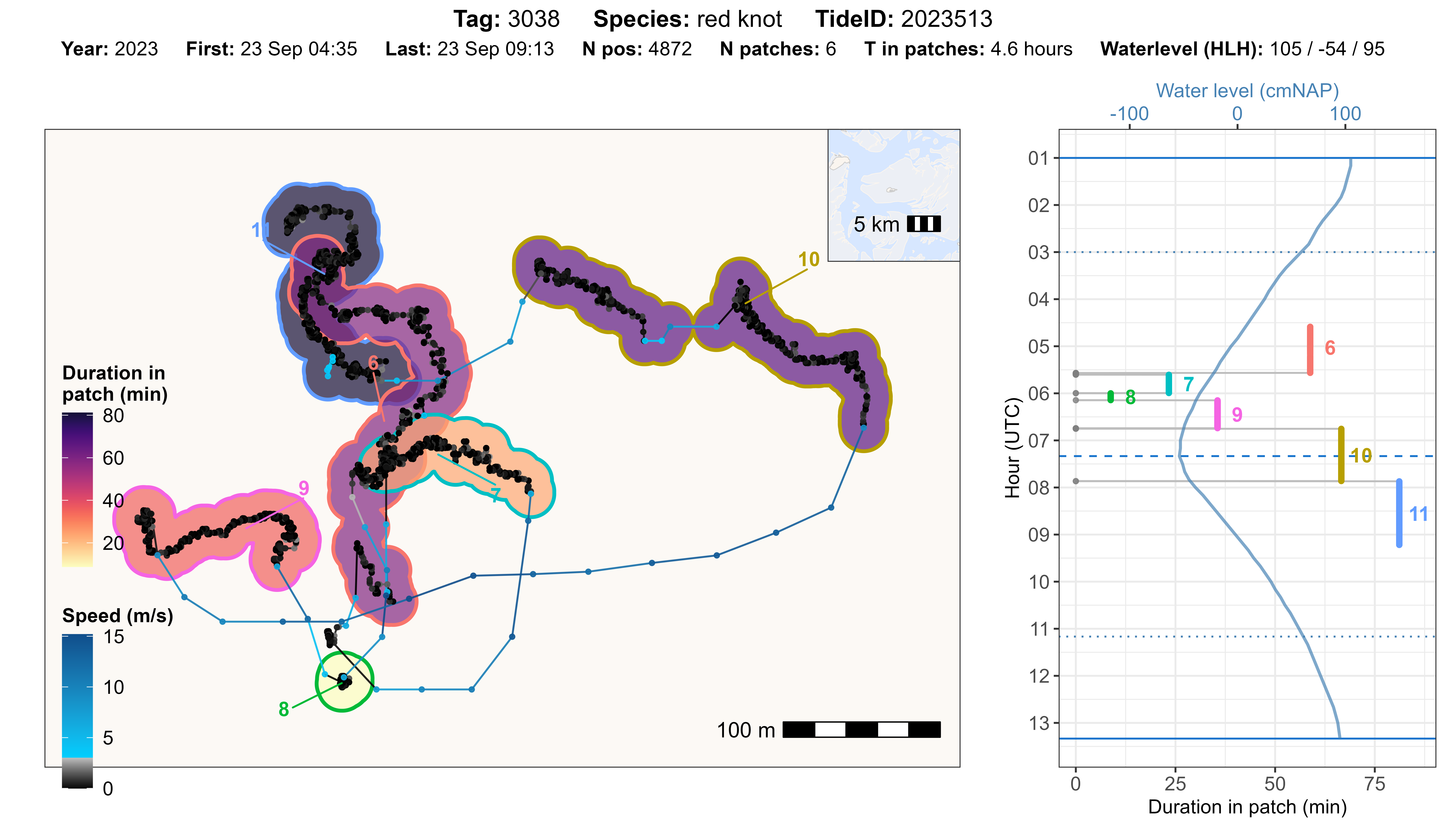
It might also be convenient to zoom in on specifc range of residence patches, to inspect them in more detail.

# set parameters for subsetting data
tag_id <- "3038"
tide_id <- "2023513"
from_patch <- 6
to_patch <- 11

atl_check_res_patch(
  data[
    tag == tag_id &
      datetime >= data[
        tag == tag_id & tideID == tide_id & patch == from_patch, min(datetime)
      ] &
      datetime <= data[
        tag == tag_id & tideID == tide_id & patch == to_patch, max(datetime)
      ]
  ],
  tide_data = tidal_pattern, tide_data_highres = measured_water_height,
  tide = tide_id, offset = 30,
  buffer_res_patches = 15,
  buffer_bm = 50,
  patch_label_padding = 2
)

Inspect many tags and tides

To get a general overview of the performance of residence patch assignment, we can also loop through and plot all data by tag and tide, or for example a random sample of 100 tags and tides. The plots can be saved in any directory (e.g. ./outputs/res_patch_check/), which has to be created before running the code.

# create table with data combinations to plot
idc <- unique(data[, c("species", "tag", "tideID")])

# sample 100 combinations to plot
set.seed(123)
idc <- idc[sample(.N, 100)]

# register cores and backend for parallel processing
registerDoFuture()
plan(multisession)

# loop to make plots for all
foreach(i = seq_len(nrow(idc))) %dofuture% {

  # plot and save for each combination
  atl_check_res_patch(
    data[tag == idc$tag[i]],
    tide_data = tidal_pattern,
    tide_data_highres = measured_water_height,
    tide = idc$tideID[i], offset = 30,
    buffer_res_patches = 75 / 2,
    filename = paste0(
      "./outputs/res_patch_check/",
      idc$species[i], "_tag_", idc$tag[i], "_tide_", idc$tideID[i]
    )
  )

}

# close parallel processing
plan(sequential)

Based on these plots and perhaps additional checks, the parameters can be adjusted to improve the assignment of residence patches. See the section below on choosing the best parameter settings.

Summary of residence patch data

Once satisfied with the residence patch assignment, we can summarize the residence patches by tag and patch ID and merge the desired columns back to our full data table.

# summary of residence patches
data_summary <- atl_res_patch_summary(data)

# standardise duration to minutes
data_summary[, duration := duration / 60]

# merge desired summary columns with original data table
data[data_summary, on = c("tag", "patch"), `:=`(
  duration = i.duration,
  disp_in_patch = i.disp_in_patch
)]

# show head of the summary table
head(data_summary) |> knitr::kable(digits = 2)

species	tag	patch	nfixes	x_mean	x_median	x_start	x_end	y_mean	y_median	y_start	y_end	time_mean	time_median	time_start	time_end	dist_start_end	dist_in_patch	dist_bw_patch	time_bw_patch	disp_in_patch	duration
redshank	3027	1	65	650705.6	650703.9	650705.6	650709.5	5902564	5902562	5902556	5902560	2023-09-23 03:40:31	2023-09-23 03:25:31	2023-09-23 03:13:25	2023-09-23 04:20:33	5.79	212.19	NA	NA	5.79	67.15
redshank	3027	2	60	650776.6	650776.6	650778.7	650771.9	5902216	5902217	5902216	5902206	2023-09-23 04:25:34	2023-09-23 04:25:32	2023-09-23 04:24:00	2023-09-23 04:27:09	12.29	51.41	351.03	206.99	12.29	3.15
redshank	3027	3	2456	650760.9	650762.0	650778.4	650699.8	5901722	5901737	5902014	5901490	2023-09-23 05:38:18	2023-09-23 05:35:44	2023-09-23 04:27:36	2023-09-23 06:51:24	530.22	1968.58	192.16	27.00	530.22	143.79
redshank	3027	4	25	648514.3	648514.8	648516.0	648514.2	5901441	5901440	5901453	5901441	2023-09-23 06:55:19	2023-09-23 06:55:21	2023-09-23 06:54:36	2023-09-23 06:55:57	11.98	37.77	2184.17	191.99	11.98	1.35
redshank	3027	5	64	648364.2	648362.5	648360.7	648365.8	5901596	5901590	5901578	5901620	2023-09-23 06:58:00	2023-09-23 06:58:01	2023-09-23 06:56:18	2023-09-23 06:59:42	42.01	79.03	206.04	21.00	42.01	3.40
redshank	3027	6	41	648059.6	648058.4	648059.7	648058.4	5902193	5902192	5902184	5902204	2023-09-23 07:01:48	2023-09-23 07:01:51	2023-09-23 07:00:39	2023-09-23 07:02:57	19.69	48.94	641.75	57.00	19.69	2.30

Here is description of the different columns in the output data table:

Column	Description
tag	4 digit tag ID (character), i.e. last 4 digits of the full tag number
patch	Patch ID
nfixes	Number of fixes in the patch
x_mean	Mean X-coordinate in meters (UTM 31 N)
x_median	Median X-coordinate in meters (UTM 31 N)
x_start	X-coordinate at the start of the residence patch (UTM 31 N)
x_end	X-coordinate at the end of the residence patch (UTM 31 N)
y_mean	Mean Y-coordinate in meters (UTM 31 N)
y_median	Median Y-coordinate in meters (UTM 31 N)
y_start	Y-coordinate at the start of the residence patch (UTM 31 N)
y_end	Y-coordinate at the end of the residence patch (UTM 31 N)
time_mean	Mean datetime of the positions in the residence patch
time_median	Median datetime of the positions in the residence patch
time_start	Start datetime of the patch
time_end	End datetime of the patch
dist_start_end	Distance (in meters) between first and last position
dist_in_patch	Distance (in meters) travelled within the patch (cumulative distance)
dist_bw_patch	Distance (in meters) between end of previous and start of current patch
time_bw_patch	Time (in seconds) between end of previous and start of current patch
disp_in_patch	Straight-line displacement (in meters) between start and end of the patch
duration	Time duration (in seconds) between first and last position in patch

Plotting residence patches

Residence patches can be conveniently plotted using ggplot2. Here, we will show plotting residence patchs by individuals or species.

Plot by individual

Here, we will provide three examples of plotting residence patches for one red knot (tag 3038).

Plot track coloured by patch ID

In the first example, the residence patches are coloured by patch ID. To show the full track, the transient (unassigned) positions are plotted in grey.

# subset red knot
data_subset <- data[tag == 3038]
data_summary_subset <- data_summary[tag == 3038]

# create basemap
bm <- atl_create_bm(data_subset, buffer = 500)

# track with residence patches coloured
bm +
  geom_path(data = data_subset, aes(x, y), alpha = 0.1) +
  geom_point(
    data = data_subset, aes(x, y), color = "grey",
    show.legend = FALSE
  ) +
  geom_point(
    data = data_subset[!is.na(patch)], aes(x, y, color = as.character(patch)),
    size = 1.5, show.legend = FALSE
  )

Plot residence patches coloured by patch ID

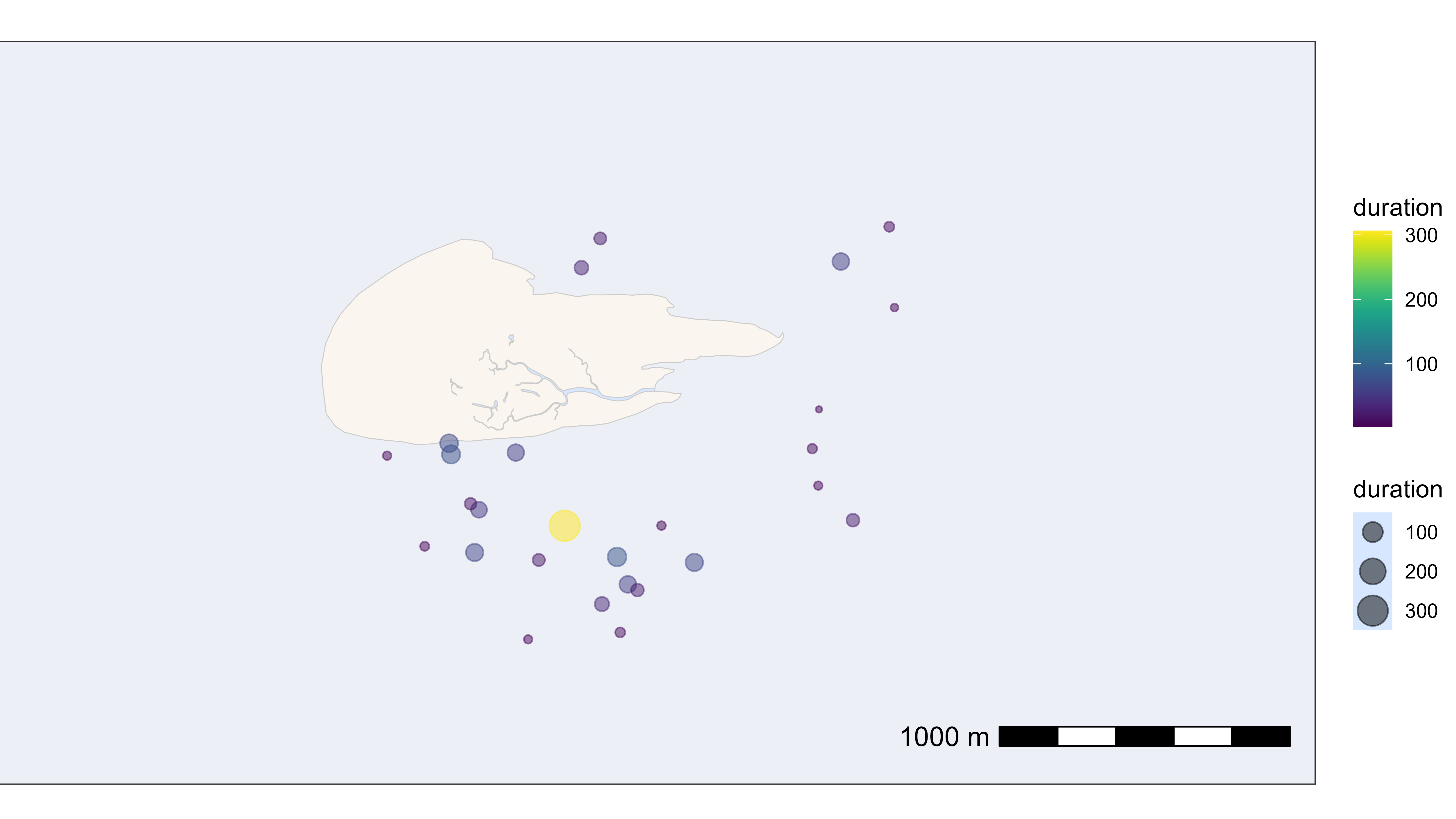
In the second example, the residence patches are plotted at their median positions with the size and colour scaled to their duration (in minutes).

# plot residence patches itself by duration
bm +
  geom_point(
    data = data_summary_subset,
    aes(x_median, y_median, color = duration, size = duration),
    show.legend = TRUE, alpha = 0.5
  ) +
  scale_color_viridis()

Plot track with residence patches as polygons

In the third example, we will calculate polygons around the residence patches and plot them

# make patch character for plotting
data_subset[, patch := as.character(patch)]

# create polygons around residence patches
d_sf <- atl_as_sf(
  data_subset,
  additional_cols = "patch",
  option = "res_patches", buffer = 75 / 2
)

# geom_sf overwrites the coordinate system, so we need to set the limits again
bbox <- atl_bbox(data_subset, buffer = 500)

# plot polygons around residence patches
bm +
  # add patch polygons
  geom_sf(data = d_sf, aes(fill = patch), alpha = 0.2) +
  # add track and points
  geom_path(
    data = data_subset, aes(x, y),
    linewidth = 0.5, alpha = 0.5
  ) +
  geom_point(
    data = data_subset[is.na(patch)], aes(x, y),
    size = 0.5, alpha = 0.5, color = "grey20",
    show.legend = FALSE
  ) +
  geom_point(
    data = data_subset[!is.na(patch)], aes(x, y, color = patch),
    size = 0.5, show.legend = FALSE
  ) +
  # set extend again (overwritten by geom_sf)
  coord_sf(
    xlim = c(bbox["xmin"], bbox["xmax"]),
    ylim = c(bbox["ymin"], bbox["ymax"]), expand = FALSE
  )

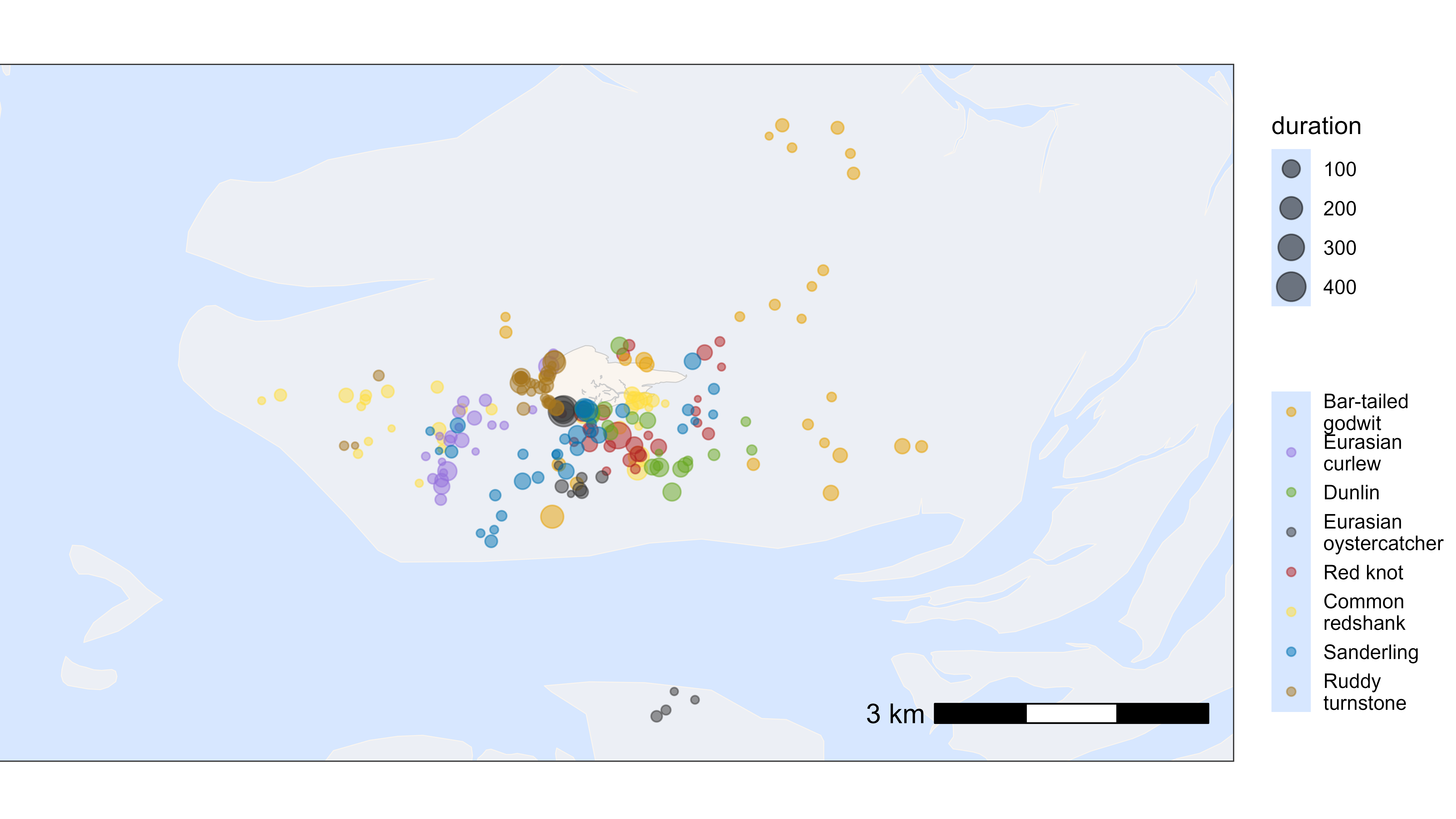
Plot by species

Similarly, we can plot the residence patches by species. For this, we need to merge the species information back to the summary table for residence patches. The residence patches are coloured by species and scaled by duration (in minutes).

# create basemap
bm <- atl_create_bm(data, buffer = 500)

# add species
du <- unique(data, by = "tag")
data_summary <- data_summary[du, on = "tag", `:=`(species = i.species)]

# plot residence patches itself by duration and species
bm +
  geom_point(
    data = data_summary,
    aes(x_median, y_median, color = species, size = duration),
    show.legend = TRUE, alpha = 0.5
  ) +
  scale_color_manual(
    values = atl_spec_cols(),
    labels = atl_spec_labs("multiline"),
    name = ""
  )

Choosing the best parameters

Selecting appropriate parameters for assigning residence patches was based on a combination of biological relevance, visual inspection, systematic testing, and expert judgement.

First, ‘min_duration’, ‘lim_time_indep’, and ‘min_fixes’ were set. To maintain biological relevance for the creation of proto-pacthes, a minimum duration of 60 s and temporal limit of 180 min were selected a-priori. Additionally, a minimum of 2 positions for a proto-patch was selected to avoid the creation of too many proto-patches with very short (biologically irrelevant) durations. These parameter settings were extensively evaluated using visual inspection.

Second, we systematically tested a range of values for two key parameters: max_speed and lim_spat_indep . Keeping all other parameters constant (see above), we varied max_speed between 2, 3, 4, and 5 m/s, and lim_spat_indep between 50, 75, and 100 m. For each combination of parameter values and for eight shorebird species tracked in the Wadden Sea in 2023, residence patches were computed for a subset of 100 randomly selected tag–tide combinations per species (with the condition that there are at least 500 positions per tag-tide combination). We then did a pair-wise comparison of parameter settings using atl_compare_res_patch_summary(), which highlighted all new, lost, merged and split residence patches. From this summary, we then selected a subset of 100 random changes that were plotted using atl_compare_res_patch_plot(). The 100 resulting plots of pair-wise comparisons were then scored by three expert observers. The observers could choose “left much better”, “left slightly better”, “similar”, “right slightly better”, or “right much better”.

Based on the systematic evaluation of parameter settings (see the figure below), a max_speed of 3 m/s and a lim_spat_indep of 75 m performed best.

Example workflow for choosing parameter values:

In this example, comparing 3 m/s and 4 m/s, the patches are wrongly merged when using 4 m/s, so the 3 m/s (left) was rated as “left much better”.

# load example data
data <- data_example

# run atl_res_patch with two different parameter sets
data_v1 <- atl_res_patch(
  data[tag == "3100"],
  max_speed = 3, lim_spat_indep = 75, lim_time_indep = 180,
  min_fixes = 2, min_duration = 60
)
data_v2 <- atl_res_patch(
  data[tag == "3100"],
  max_speed = 4, lim_spat_indep = 75, lim_time_indep = 180,
  min_fixes = 2, min_duration = 60
)

# change summary
change_summary <- atl_compare_res_patch_summary(data_v1, data_v2)

## === Patch changes summary ===
## Lost    (v1 patches gone in v2) : 0 
## Gained  (new patches in v2)     : 0 
## 
## Splits  (one v1 -> multiple v2): 0 
## Merges  (multiple v1 -> one v2): 1

# plot specific change
i <- 1

atl_compare_res_patch_plot(
  data_v1 = data_v1,
  data_v2 = data_v2,
  tag = change_summary$tag[i],
  change = change_summary$change[i],
  patch_v1 = change_summary$patch_v1[i],
  patch_v2 = change_summary$patch_v2[i]
)